class: center, middle, inverse, title-slide .title[ # Data and visualisation ] .subtitle[ ## <br><br> Data Science in a Box ] .author[ ### <a href="https://datasciencebox.org/">datasciencebox.org</a> ] --- layout: true <div class="my-footer"> <span> <a href="https://datasciencebox.org" target="_blank">datasciencebox.org</a> </span> </div> --- class: middle # What is in a dataset? 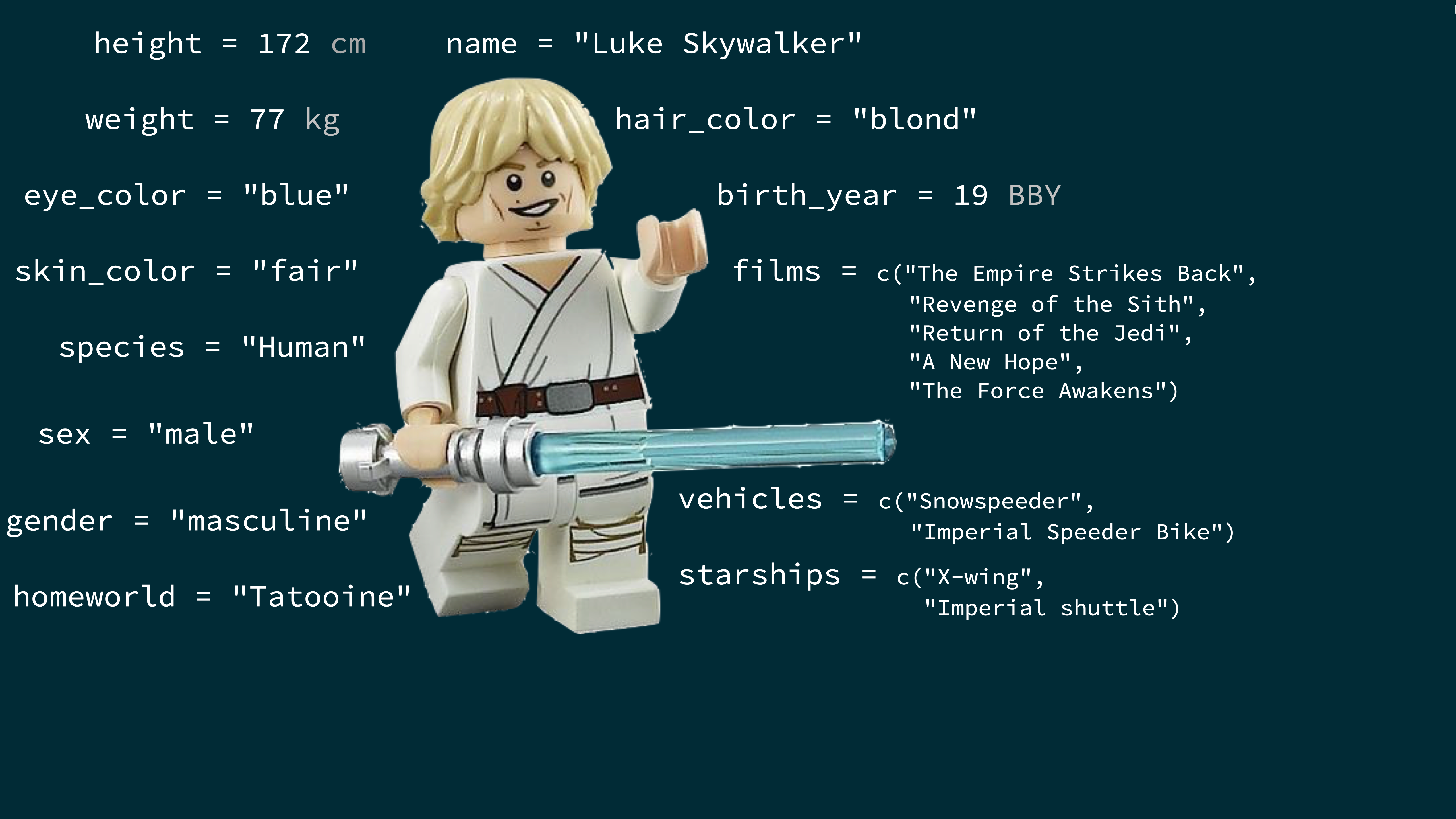--- ## Dataset terminology - Each row is an **observation** - Each column is a **variable** .small[ ```r starwars ``` ``` ## # A tibble: 87 × 14 ## name height mass hair_color skin_color eye_color birth_year ## <chr> <int> <dbl> <chr> <chr> <chr> <dbl> ## 1 Luke S… 172 77 blond fair blue 19 ## 2 C-3PO 167 75 <NA> gold yellow 112 ## 3 R2-D2 96 32 <NA> white, bl… red 33 ## 4 Darth … 202 136 none white yellow 41.9 ## 5 Leia O… 150 49 brown light brown 19 ## 6 Owen L… 178 120 brown, gr… light blue 52 ## # … with 81 more rows, and 7 more variables: sex <chr>, ## # gender <chr>, homeworld <chr>, species <chr>, films <list>, ## # vehicles <list>, starships <list> ``` ] --- ## Luke Skywalker  --- ## What's in the Star Wars data? Take a `glimpse` at the data: ```r glimpse(starwars) ``` ``` ## Rows: 87 ## Columns: 14 ## $ name <chr> "Luke Skywalker", "C-3PO", "R2-D2", "Darth V… ## $ height <int> 172, 167, 96, 202, 150, 178, 165, 97, 183, 1… ## $ mass <dbl> 77.0, 75.0, 32.0, 136.0, 49.0, 120.0, 75.0, … ## $ hair_color <chr> "blond", NA, NA, "none", "brown", "brown, gr… ## $ skin_color <chr> "fair", "gold", "white, blue", "white", "lig… ## $ eye_color <chr> "blue", "yellow", "red", "yellow", "brown", … ## $ birth_year <dbl> 19.0, 112.0, 33.0, 41.9, 19.0, 52.0, 47.0, N… ## $ sex <chr> "male", "none", "none", "male", "female", "m… ## $ gender <chr> "masculine", "masculine", "masculine", "masc… ## $ homeworld <chr> "Tatooine", "Tatooine", "Naboo", "Tatooine",… ## $ species <chr> "Human", "Droid", "Droid", "Human", "Human",… ## $ films <list> <"The Empire Strikes Back", "Revenge of the… ## $ vehicles <list> <"Snowspeeder", "Imperial Speeder Bike">, <… ## $ starships <list> <"X-wing", "Imperial shuttle">, <>, <>, "TI… ``` --- .question[ How many rows and columns does this dataset have? What does each row represent? What does each column represent? ] ```r ?starwars ``` <img src="img/starwars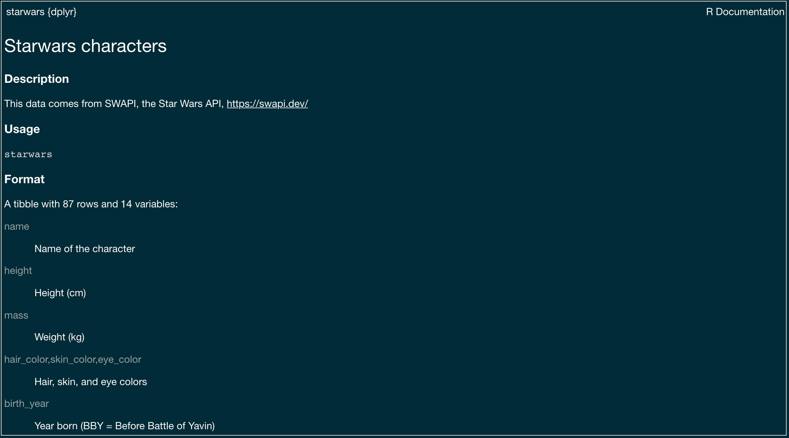-help.png" width="60%" style="display: block; margin: auto;" /> --- .question[ How many rows and columns does this dataset have? ] .pull-left[ ```r nrow(starwars) # number of rows ``` ``` ## [1] 87 ``` ```r ncol(starwars) # number of columns ``` ``` ## [1] 14 ``` ```r dim(starwars) # dimensions (row column) ``` ``` ## [1] 87 14 ``` ] --- class: middle # Exploratory data analysis --- ## What is EDA? - Exploratory data analysis (EDA) is an approach to analysing data sets to summarize its main characteristics - Often, this is visual -- this is what we'll focus on first - But we might also calculate summary statistics and perform data wrangling/manipulation/transformation at (or before) this stage of the analysis -- this is what we'll focus on next --- ## Mass vs. 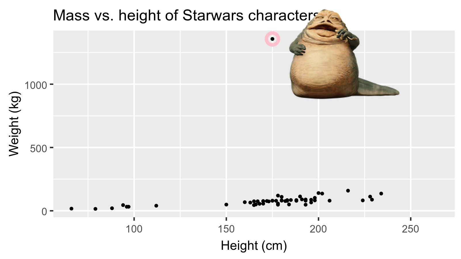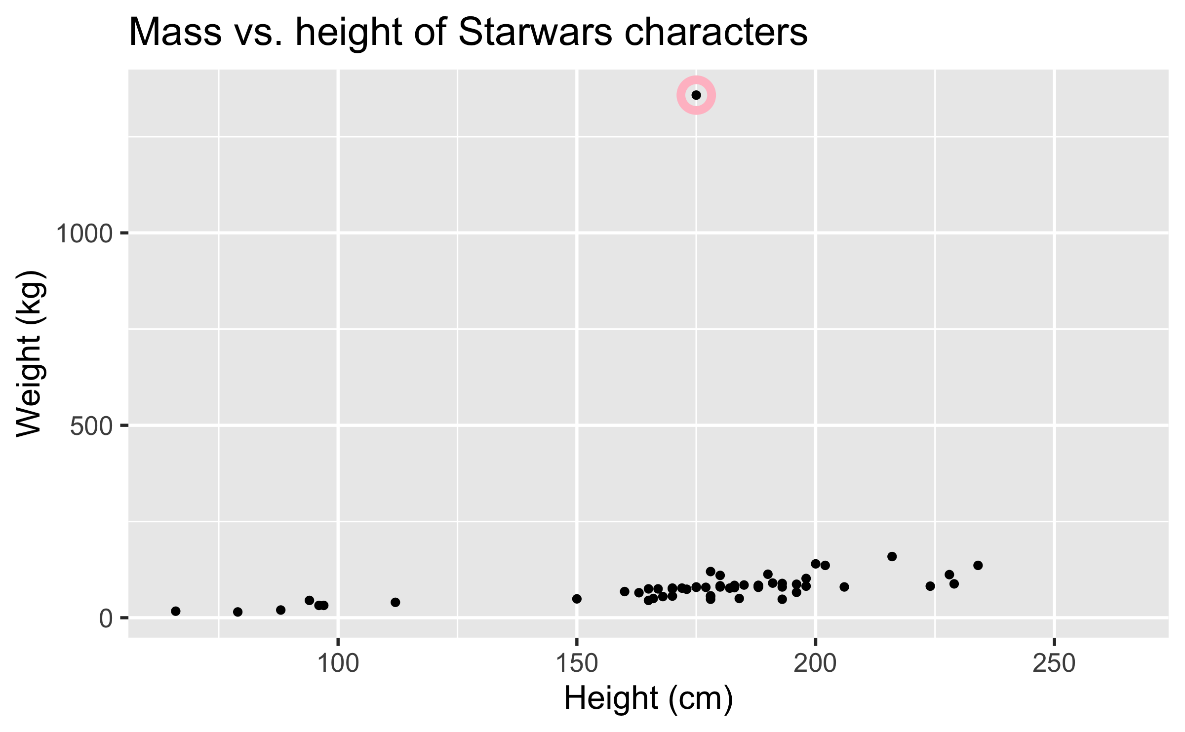height .question[ How would you describe the relationship between mass and height of Starwars characters? What other variables would help us understand data points that don't follow the overall trend? Who is the not so tall but really chubby character? ] <img src="u2-d01-data-viz_files/figure-html/unnamed-chunk-7-1.png" width="50%" style="display: block; margin: auto;" /> --- ## Jabba! <img src="img/jabbaplot.png" width="80%" style="display: block; margin: auto;" /> --- class: middle # Data visualization --- ## Data visualization > *"The simple graph has brought more information to the data analyst's mind than any other device." --- John Tukey* - Data visualization is the creation and study of the visual representation of data - Many tools for visualizing data -- R is one of them - Many approaches/systems within R for making data visualizations -- **ggplot2** is one of them, and that's what we're going to use --- ## ggplot2 `\(\in\)` tidyverse .pull-left[ <img src="img/ggplot2-part-of-tidyverse.png" width="80%" style="display: block; margin: auto;" /> ] .pull-right[ - **ggplot2** is tidyverse's data visualization package - `gg` in "ggplot2" stands for Grammar of Graphics - Inspired by the book **Grammar of Graphics** by Leland Wilkinson ] --- ## Grammar of Graphics .pull-left-narrow[ A grammar of graphics is a tool that enables us to concisely describe the components of a graphic ] .pull-right-wide[ <img src="img/grammar-of-graphics.png" width="100%" style="display: block; margin: auto;" /> ] .footnote[ 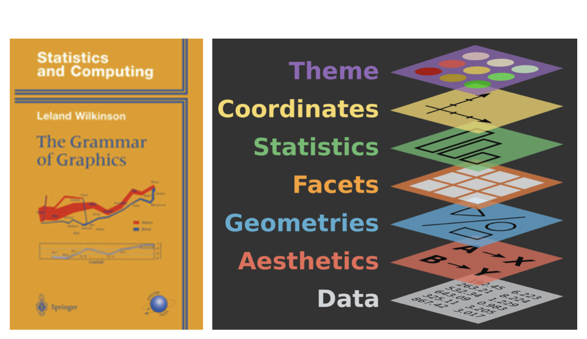Source: [BloggoType](http://bloggotype.blogspot.com/2016/08/holiday-notes2-grammar-of-graphics.html)] --- ## Mass vs. height ```r ggplot(data = starwars, mapping = aes(x = height, y = mass)) + geom_point() + labs(title = "Mass vs. height of Starwars characters", x = "Height (cm)", y = "Weight (kg)") ``` ``` ## Warning: Removed 28 rows containing missing values (geom_point).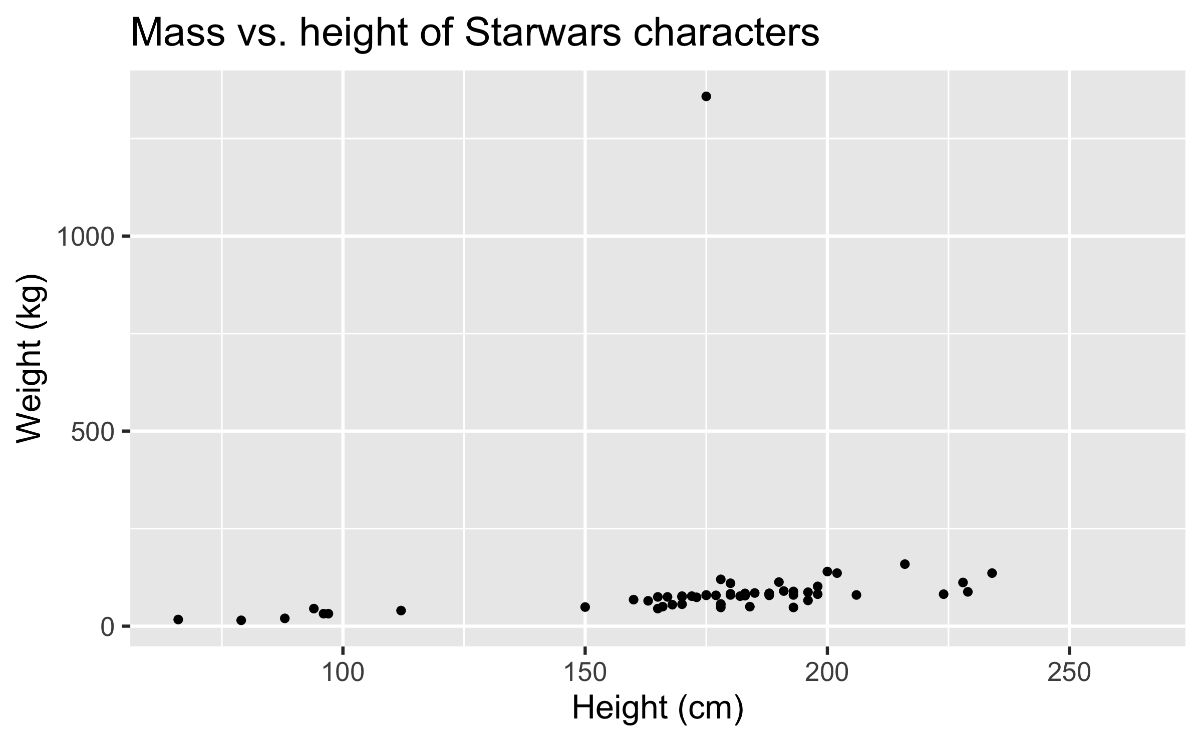 ``` <img src="u2-d01-data-viz_files/figure-html/mass-height-1.png" width="50%" style="display: block; margin: auto;" /> --- .question[ - What are the functions doing the plotting? - What is the dataset being plotted? - Which variables map to which features (aesthetics) of the plot? - What does the warning mean?⁺ ] ```r ggplot(data = starwars, mapping = aes(x = height, y = mass)) + geom_point() + labs(title = "Mass vs. height of Starwars characters", x = "Height (cm)", y = "Weight (kg)") ``` ``` ## Warning: Removed 28 rows containing missing values (geom_point). ``` .footnote[ ⁺Suppressing warning to subsequent slides to save space ] --- ## Hello ggplot2! .pull-left-wide[ - `ggplot()` is the main function in ggplot2 - Plots are constructed in layers - Structure of the code for plots can be summarized as ```r ggplot(data = [dataset], mapping = aes(x = [x-variable], y = [y-variable])) + geom_xxx() + other options ``` - The ggplot2 package comes with the tidyverse ```r library(tidyverse) ``` - For help with ggplot2, see [ggplot2.tidyverse.org](http://ggplot2.tidyverse.org/) ] --- class: middle # Why do we visualize? 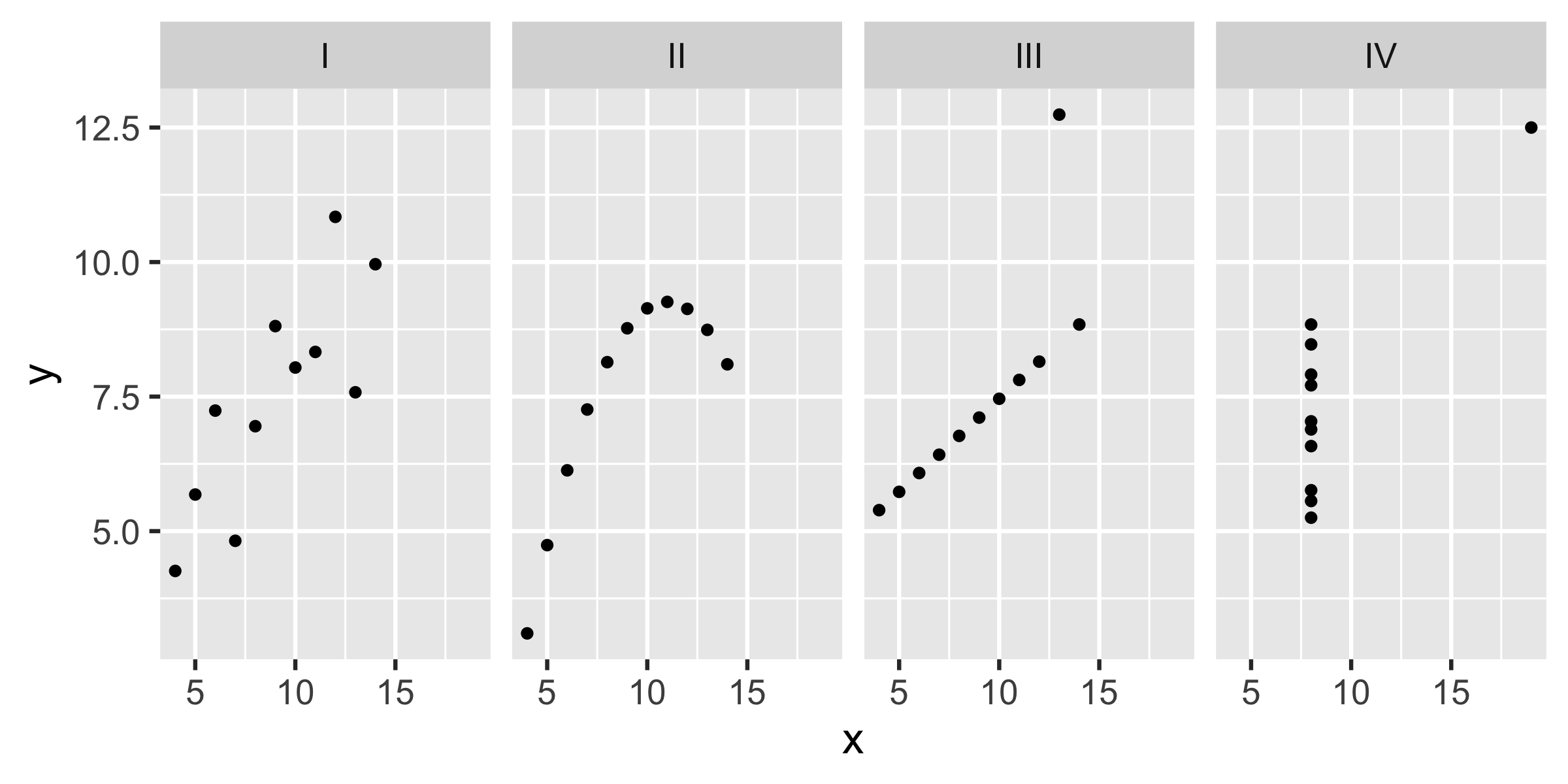--- ## Anscombe's quartet .pull-left[ ``` ## set x y ## 1 I 10 8.04 ## 2 I 8 6.95 ## 3 I 13 7.58 ## 4 I 9 8.81 ## 5 I 11 8.33 ## 6 I 14 9.96 ## 7 I 6 7.24 ## 8 I 4 4.26 ## 9 I 12 10.84 ## 10 I 7 4.82 ## 11 I 5 5.68 ## 12 II 10 9.14 ## 13 II 8 8.14 ## 14 II 13 8.74 ## 15 II 9 8.77 ## 16 II 11 9.26 ## 17 II 14 8.10 ## 18 II 6 6.13 ## 19 II 4 3.10 ## 20 II 12 9.13 ## 21 II 7 7.26 ## 22 II 5 4.74 ``` ] .pull-right[ ``` ## set x y ## 23 III 10 7.46 ## 24 III 8 6.77 ## 25 III 13 12.74 ## 26 III 9 7.11 ## 27 III 11 7.81 ## 28 III 14 8.84 ## 29 III 6 6.08 ## 30 III 4 5.39 ## 31 III 12 8.15 ## 32 III 7 6.42 ## 33 III 5 5.73 ## 34 IV 8 6.58 ## 35 IV 8 5.76 ## 36 IV 8 7.71 ## 37 IV 8 8.84 ## 38 IV 8 8.47 ## 39 IV 8 7.04 ## 40 IV 8 5.25 ## 41 IV 19 12.50 ## 42 IV 8 5.56 ## 43 IV 8 7.91 ## 44 IV 8 6.89 ``` ] --- ## Summarising Anscombe's quartet ```r quartet %>% group_by(set) %>% summarise( mean_x = mean(x), mean_y = mean(y), sd_x = sd(x), sd_y = sd(y), r = cor(x, y) ) ``` ``` ## # A tibble: 4 × 6 ## set mean_x mean_y sd_x sd_y r ## <fct> <dbl> <dbl> <dbl> <dbl> <dbl> ## 1 I 9 7.50 3.32 2.03 0.816 ## 2 II 9 7.50 3.32 2.03 0.816 ## 3 III 9 7.5 3.32 2.03 0.816 ## 4 IV 9 7.50 3.32 2.03 0.817 ``` --- ## Visualizing Anscombe's quartet <img src="u2-d01-data-viz_files/figure-html/quartet-plot-1.png" width="80%" style="display: block; margin: auto;" /> --- ## Age at first kiss .question[ Do you see anything out of the ordinary? 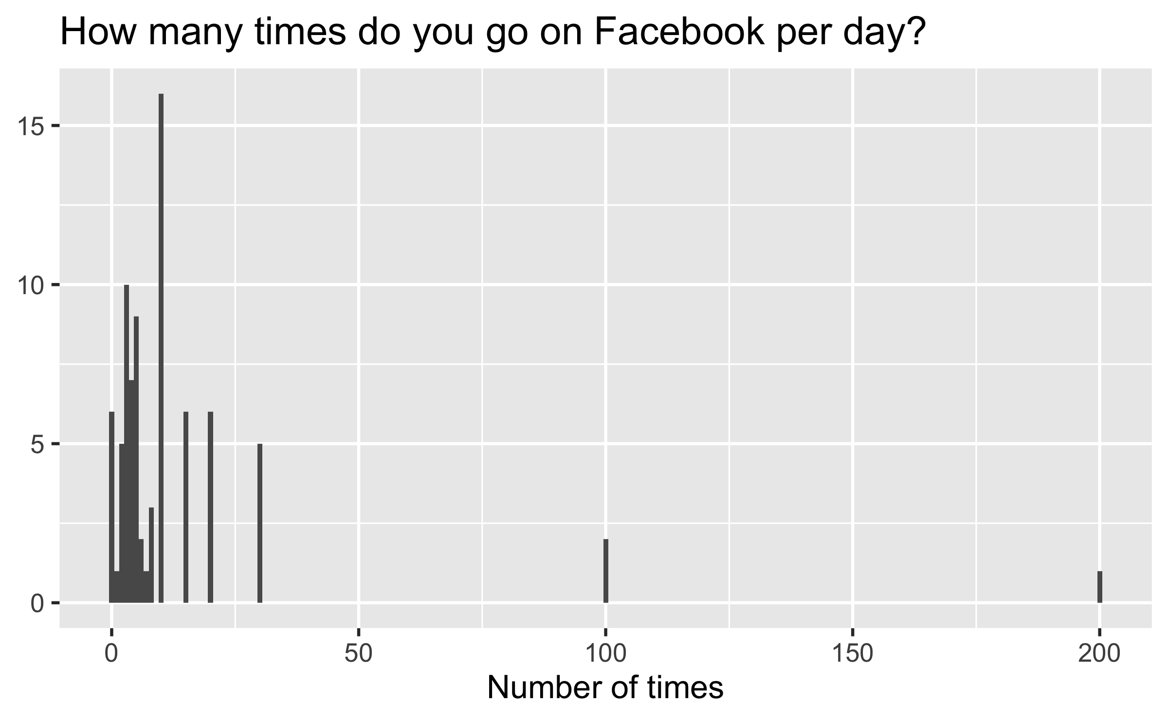] <img src="u2-d01-data-viz_files/figure-html/unnamed-chunk-14-1.png" width="60%" style="display: block; margin: auto;" /> --- ## Facebook visits .question[ How are people reporting lower vs. higher values of FB visits? ] <img src="u2-d01-data-viz_files/figure-html/unnamed-chunk-15-1.png" width="60%" style="display: block; margin: auto;" />