ggplot2 ∈ tidyverse
- ggplot2 is tidyverse's data visualization package
- Structure of the code for plots can be summarized as
ggplot(data = [dataset], mapping = aes(x = [x-variable], y = [y-variable])) + geom_xxx() + other optionsData: Palmer Penguins
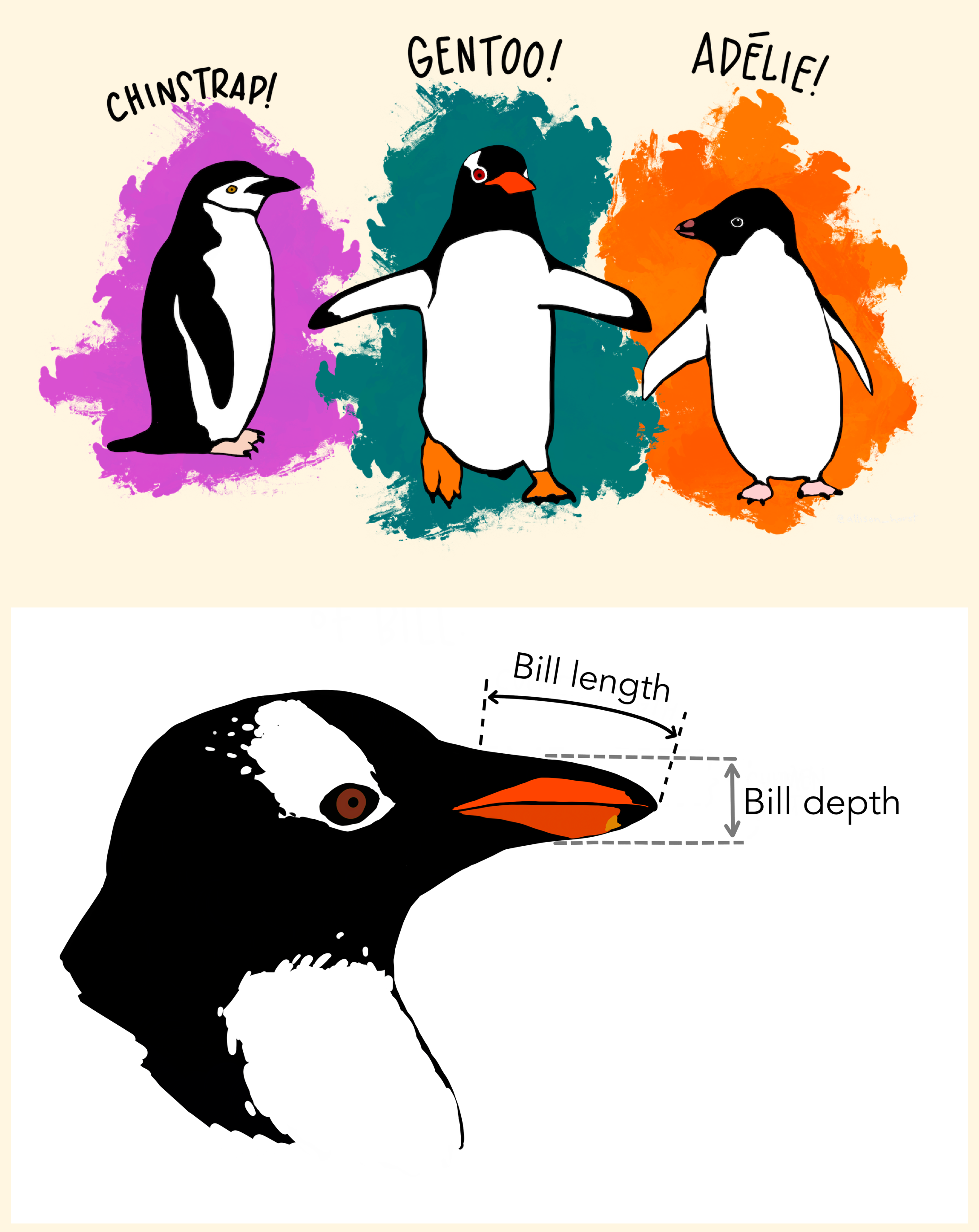
Measurements for penguin species, island in Palmer Archipelago, size (flipper length, body mass, bill dimensions), and sex.
library(palmerpenguins)glimpse(penguins)## Rows: 344## Columns: 8## $ species <fct> Adelie, Adelie, Adelie, Adelie, Adeli…## $ island <fct> Torgersen, Torgersen, Torgersen, Torg…## $ bill_length_mm <dbl> 39.1, 39.5, 40.3, NA, 36.7, 39.3, 38.…## $ bill_depth_mm <dbl> 18.7, 17.4, 18.0, NA, 19.3, 20.6, 17.…## $ flipper_length_mm <int> 181, 186, 195, NA, 193, 190, 181, 195…## $ body_mass_g <int> 3750, 3800, 3250, NA, 3450, 3650, 362…## $ sex <fct> male, female, female, NA, female, mal…## $ year <int> 2007, 2007, 2007, 2007, 2007, 2007, 2…

ggplot(data = penguins, mapping = aes(x = bill_depth_mm, y = bill_length_mm, colour = species)) + geom_point() + labs(title = "Bill depth and length", subtitle = "Dimensions for Adelie, Chinstrap, and Gentoo Penguins", x = "Bill depth (mm)", y = "Bill length (mm)", colour = "Species")## Warning: Removed 2 rows containing missing values (geom_point).Start with the
penguinsdata frame, map bill depth to the x-axis
ggplot(data = penguins, mapping = aes(x = bill_depth_mm))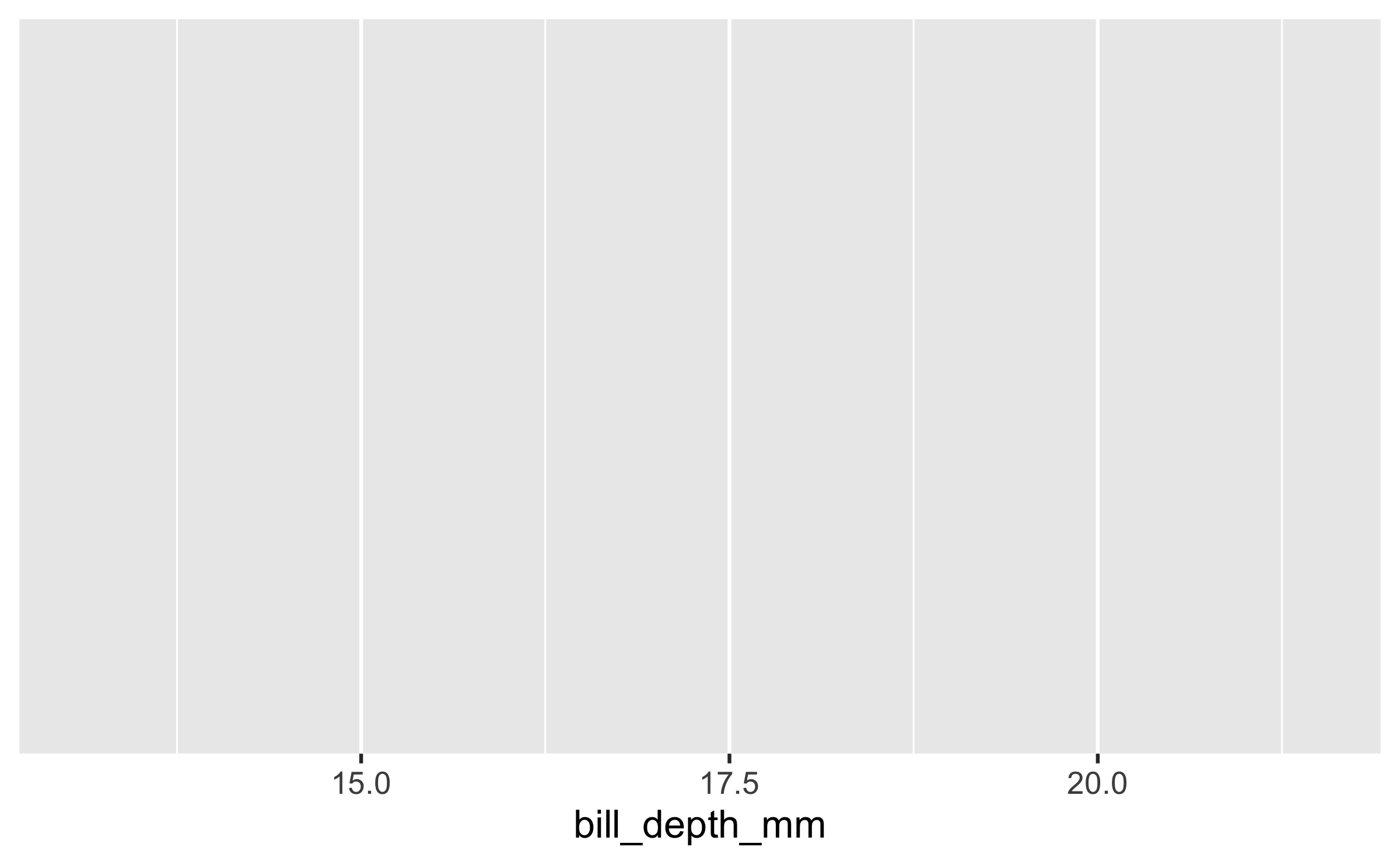
Start with the
penguinsdata frame, map bill depth to the x-axis and map bill length to the y-axis.
ggplot(data = penguins, mapping = aes(x = bill_depth_mm, y = bill_length_mm))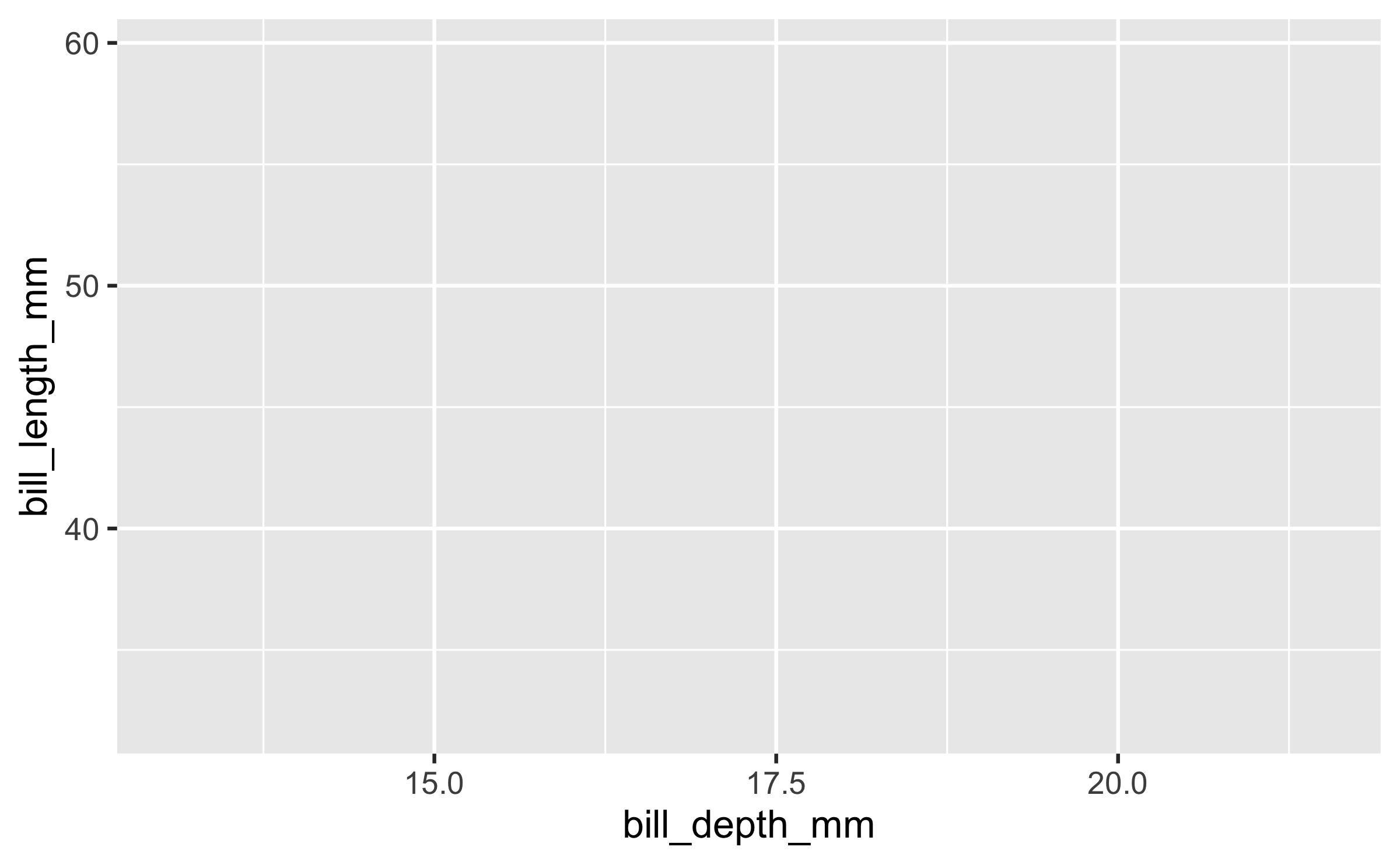
Start with the
penguinsdata frame, map bill depth to the x-axis and map bill length to the y-axis. Represent each observation with a point
ggplot(data = penguins, mapping = aes(x = bill_depth_mm, y = bill_length_mm)) + geom_point()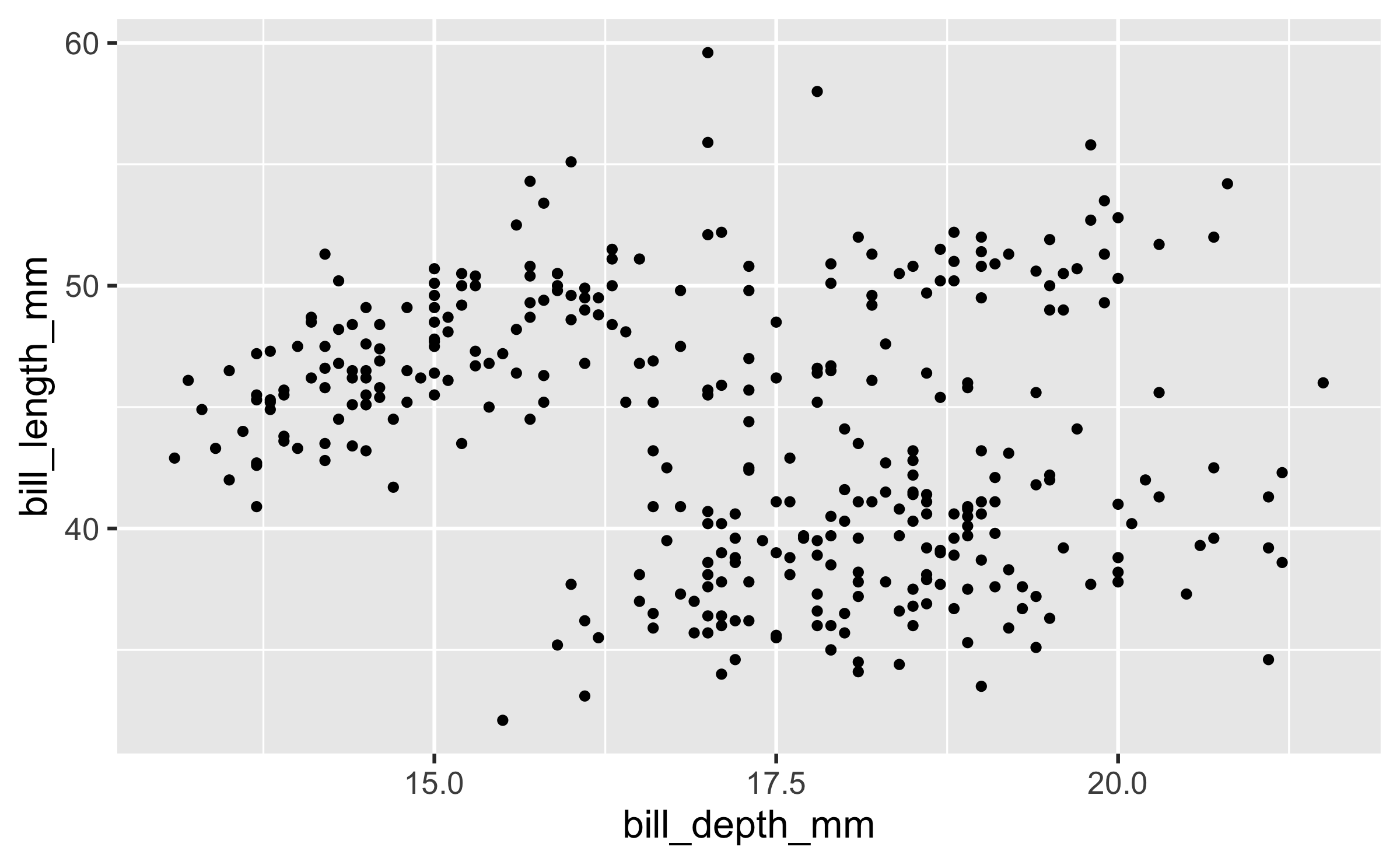
Start with the
penguinsdata frame, map bill depth to the x-axis and map bill length to the y-axis. Represent each observation with a point and map species to the colour of each point.
ggplot(data = penguins, mapping = aes(x = bill_depth_mm, y = bill_length_mm, colour = species)) + geom_point()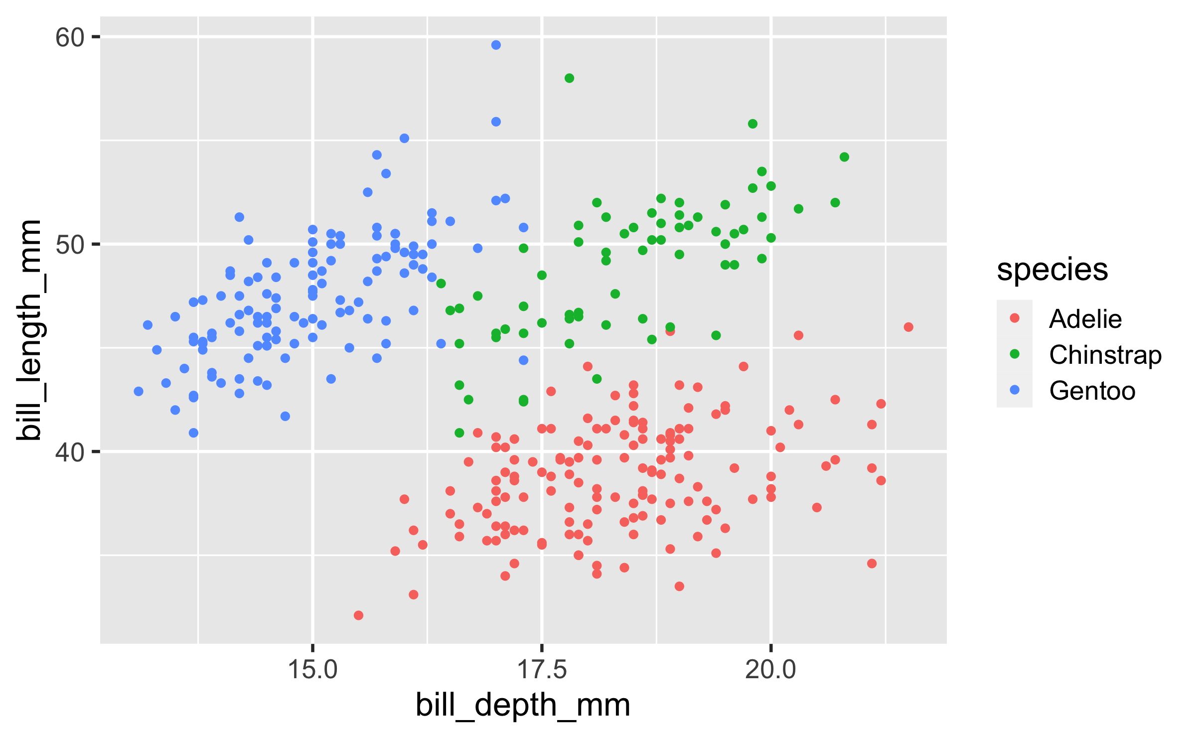
Start with the
penguinsdata frame, map bill depth to the x-axis and map bill length to the y-axis. Represent each observation with a point and map species to the colour of each point. Title the plot "Bill depth and length"
ggplot(data = penguins, mapping = aes(x = bill_depth_mm, y = bill_length_mm, colour = species)) + geom_point() + labs(title = "Bill depth and length")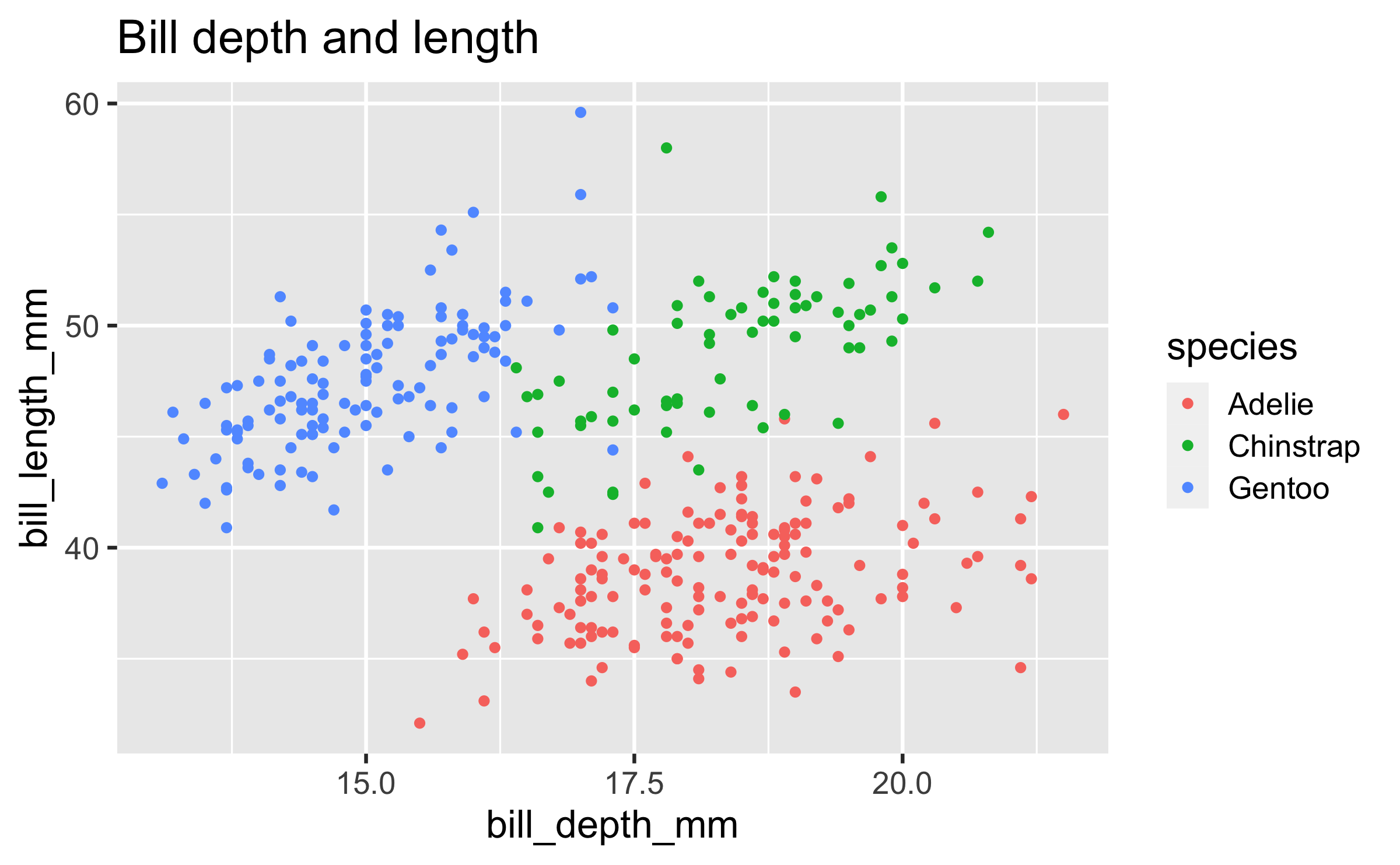
Start with the
penguinsdata frame, map bill depth to the x-axis and map bill length to the y-axis. Represent each observation with a point and map species to the colour of each point. Title the plot "Bill depth and length", add the subtitle "Dimensions for Adelie, Chinstrap, and Gentoo Penguins"
ggplot(data = penguins, mapping = aes(x = bill_depth_mm, y = bill_length_mm, colour = species)) + geom_point() + labs(title = "Bill depth and length", subtitle = "Dimensions for Adelie, Chinstrap, and Gentoo Penguins")
Start with the
penguinsdata frame, map bill depth to the x-axis and map bill length to the y-axis. Represent each observation with a point and map species to the colour of each point. Title the plot "Bill depth and length", add the subtitle "Dimensions for Adelie, Chinstrap, and Gentoo Penguins", label the x and y axes as "Bill depth (mm)" and "Bill length (mm)", respectively
ggplot(data = penguins, mapping = aes(x = bill_depth_mm, y = bill_length_mm, colour = species)) + geom_point() + labs(title = "Bill depth and length", subtitle = "Dimensions for Adelie, Chinstrap, and Gentoo Penguins", x = "Bill depth (mm)", y = "Bill length (mm)")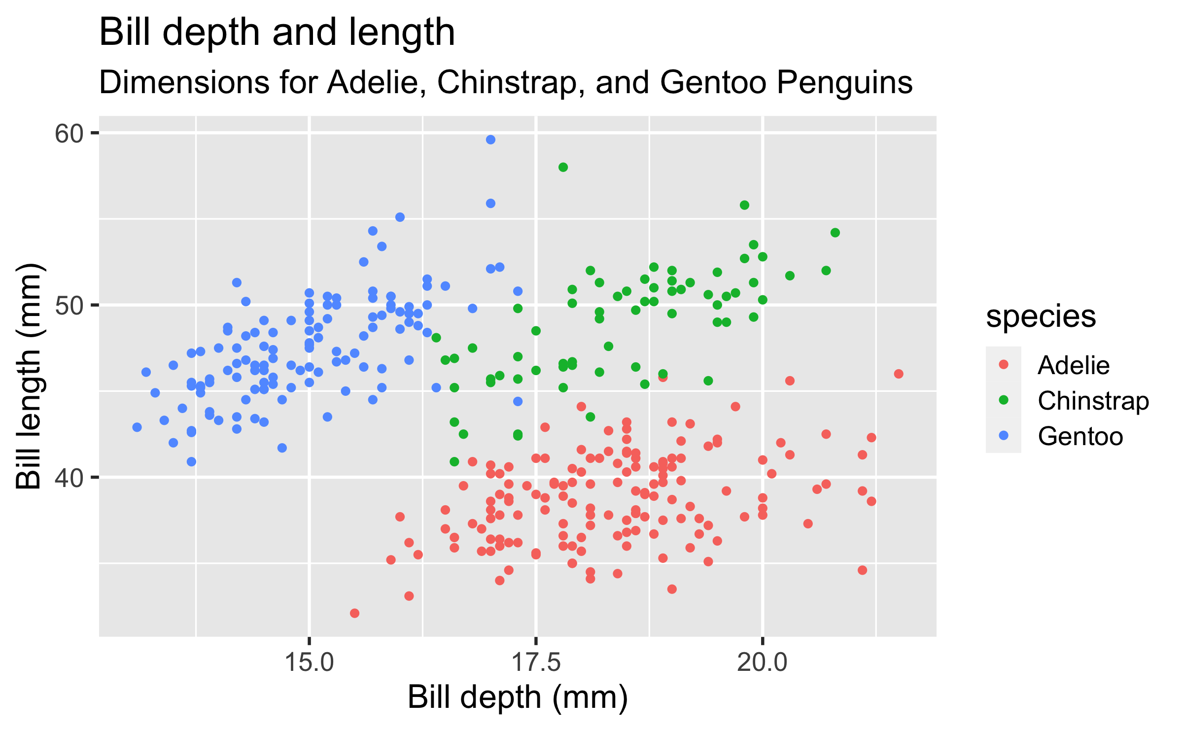
Start with the
penguinsdata frame, map bill depth to the x-axis and map bill length to the y-axis. Represent each observation with a point and map species to the colour of each point. Title the plot "Bill depth and length", add the subtitle "Dimensions for Adelie, Chinstrap, and Gentoo Penguins", label the x and y axes as "Bill depth (mm)" and "Bill length (mm)", respectively, label the legend "Species"
ggplot(data = penguins, mapping = aes(x = bill_depth_mm, y = bill_length_mm, colour = species)) + geom_point() + labs(title = "Bill depth and length", subtitle = "Dimensions for Adelie, Chinstrap, and Gentoo Penguins", x = "Bill depth (mm)", y = "Bill length (mm)", colour = "Species")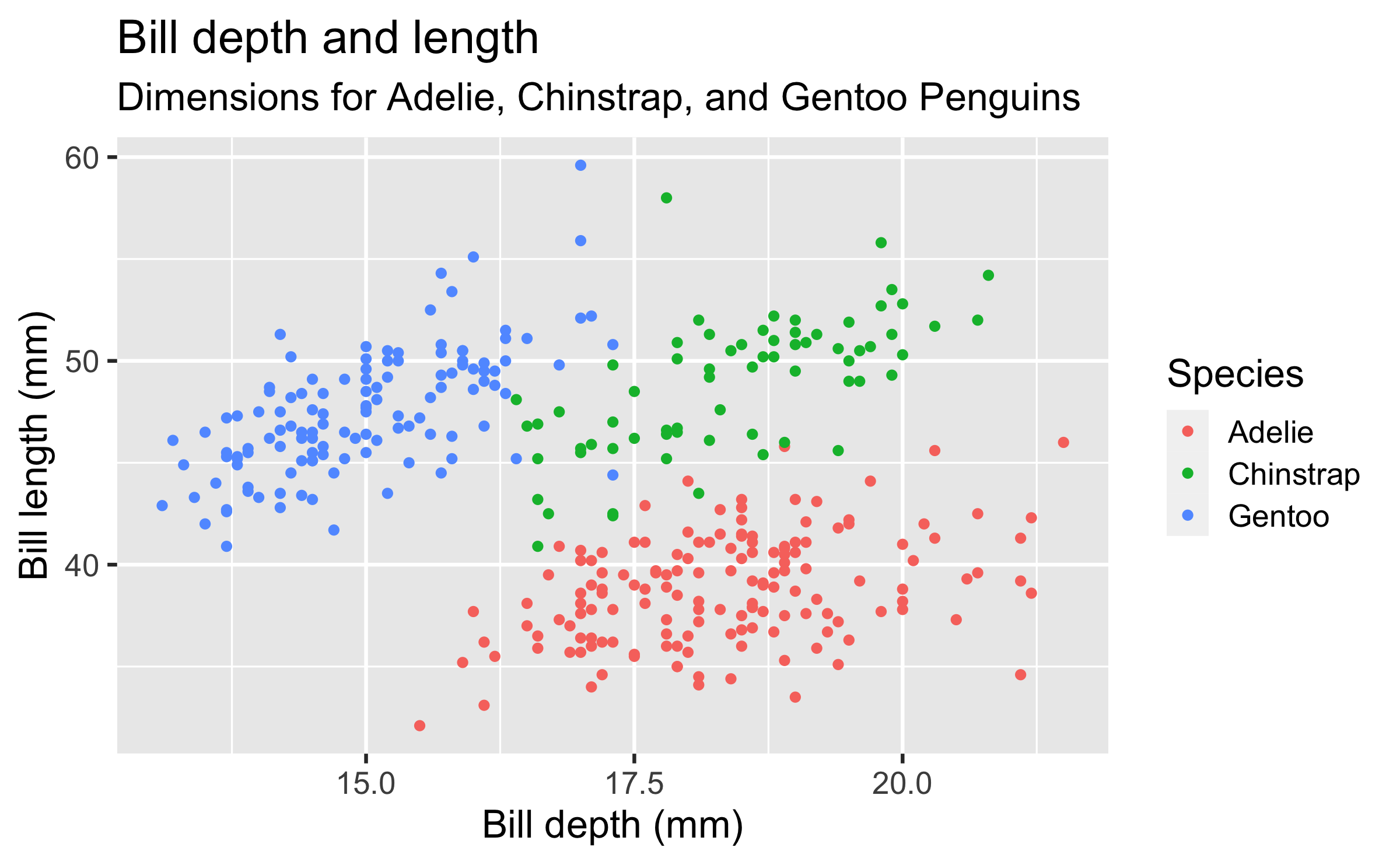
Start with the
penguinsdata frame, map bill depth to the x-axis and map bill length to the y-axis. Represent each observation with a point and map species to the colour of each point. Title the plot "Bill depth and length", add the subtitle "Dimensions for Adelie, Chinstrap, and Gentoo Penguins", label the x and y axes as "Bill depth (mm)" and "Bill length (mm)", respectively, label the legend "Species", and add a caption for the data source.
ggplot(data = penguins, mapping = aes(x = bill_depth_mm, y = bill_length_mm, colour = species)) + geom_point() + labs(title = "Bill depth and length", subtitle = "Dimensions for Adelie, Chinstrap, and Gentoo Penguins", x = "Bill depth (mm)", y = "Bill length (mm)", colour = "Species", caption = "Source: Palmer Station LTER / palmerpenguins package")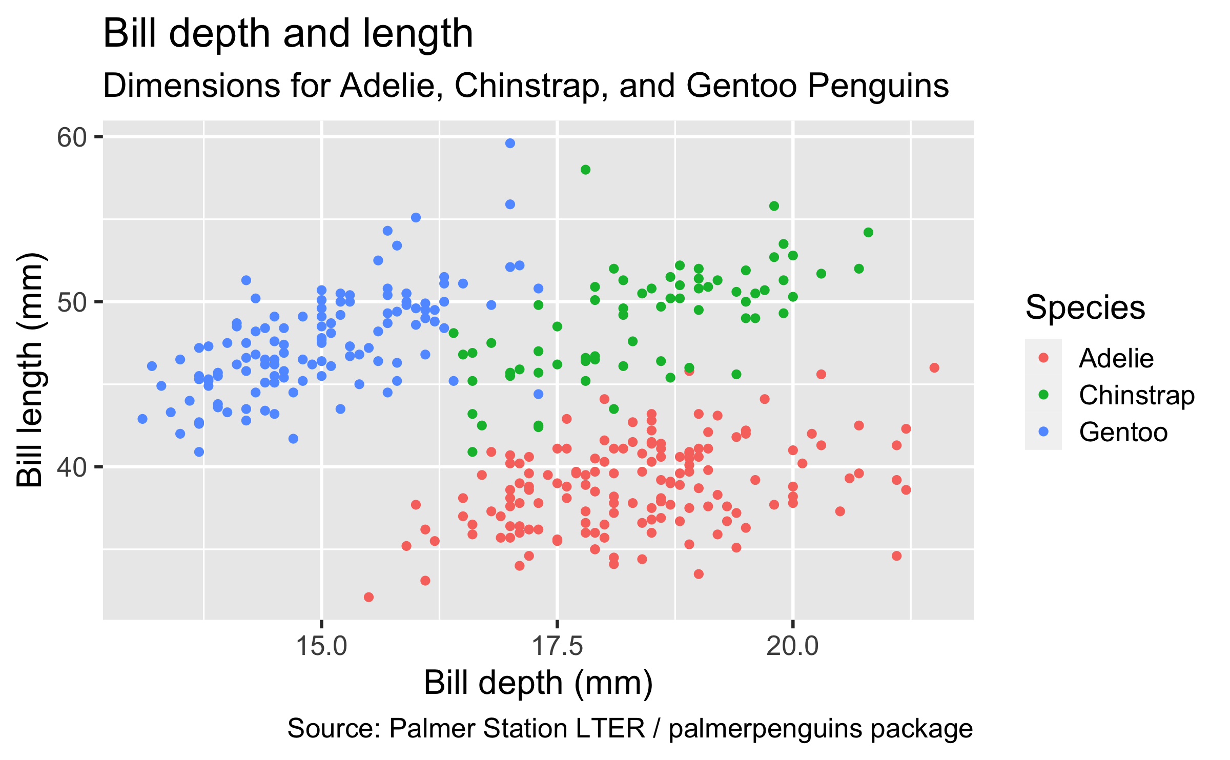
Start with the
penguinsdata frame, map bill depth to the x-axis and map bill length to the y-axis. Represent each observation with a point and map species to the colour of each point. Title the plot "Bill depth and length", add the subtitle "Dimensions for Adelie, Chinstrap, and Gentoo Penguins", label the x and y axes as "Bill depth (mm)" and "Bill length (mm)", respectively, label the legend "Species", and add a caption for the data source. Finally, use a discrete colour scale that is designed to be perceived by viewers with common forms of colour blindness.
ggplot(data = penguins, mapping = aes(x = bill_depth_mm, y = bill_length_mm, colour = species)) + geom_point() + labs(title = "Bill depth and length", subtitle = "Dimensions for Adelie, Chinstrap, and Gentoo Penguins", x = "Bill depth (mm)", y = "Bill length (mm)", colour = "Species", caption = "Source: Palmer Station LTER / palmerpenguins package") + scale_colour_viridis_d()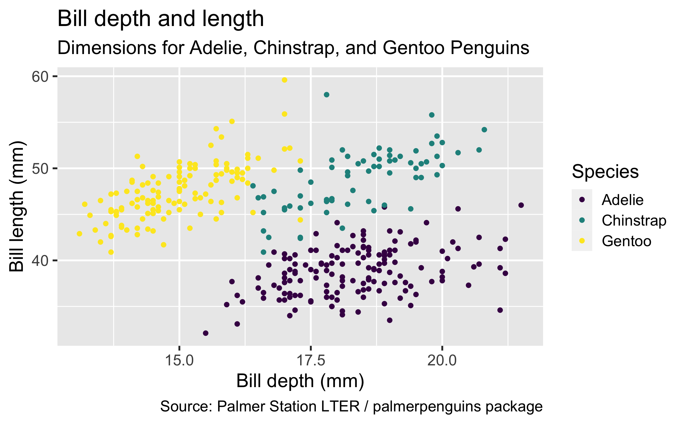

ggplot(data = penguins, mapping = aes(x = bill_depth_mm, y = bill_length_mm, colour = species)) + geom_point() + labs(title = "Bill depth and length", subtitle = "Dimensions for Adelie, Chinstrap, and Gentoo Penguins", x = "Bill depth (mm)", y = "Bill length (mm)", colour = "Species", caption = "Source: Palmer Station LTER / palmerpenguins package") + scale_colour_viridis_d()## Warning: Removed 2 rows containing missing values (geom_point).Start with the penguins data frame,
map bill depth to the x-axis
and map bill length to the y-axis.
Represent each observation with a point and map species to the colour of each point.
Title the plot "Bill depth and length", add the subtitle "Dimensions for Adelie, Chinstrap, and Gentoo Penguins", label the x and y axes as "Bill depth (mm)" and "Bill length (mm)", respectively, label the legend "Species", and add a caption for the data source.
Finally, use a discrete colour scale that is designed to be perceived by viewers with common forms of colour blindness.
Argument names
You can omit the names of first two arguments when building plots with ggplot().
ggplot(data = penguins, mapping = aes(x = bill_depth_mm, y = bill_length_mm, colour = species)) + geom_point() + scale_colour_viridis_d()ggplot(penguins, aes(x = bill_depth_mm, y = bill_length_mm, colour = species)) + geom_point() + scale_colour_viridis_d()Aesthetics options
Commonly used characteristics of plotting characters that can be mapped to a specific variable in the data are
colourshapesizealpha(transparency)
Colour
ggplot(penguins, aes(x = bill_depth_mm, y = bill_length_mm, colour = species)) + geom_point() + scale_colour_viridis_d()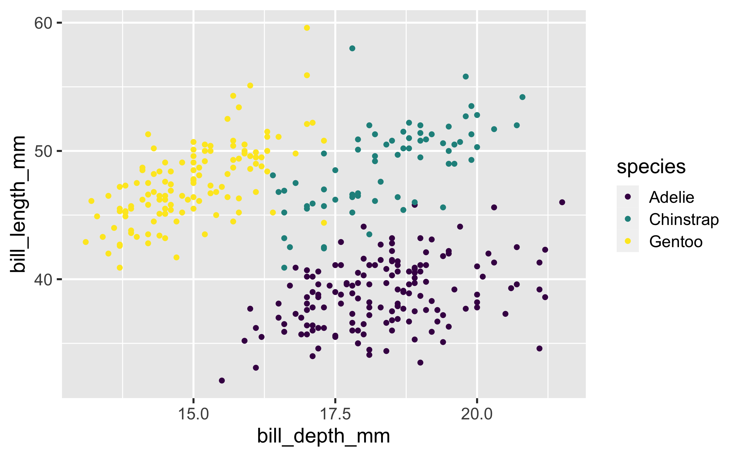
Shape
Mapped to a different variable than colour
ggplot(penguins, aes(x = bill_depth_mm, y = bill_length_mm, colour = species, shape = island)) + geom_point() + scale_colour_viridis_d()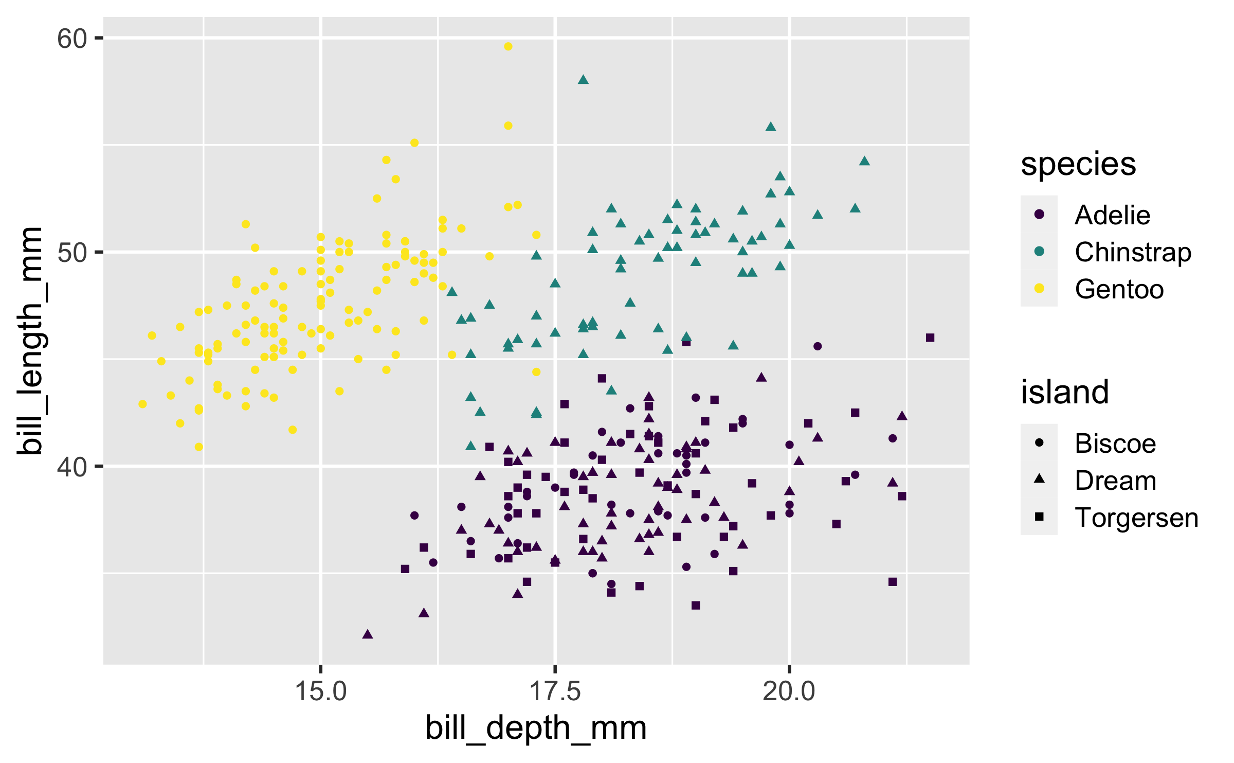
Shape
Mapped to same variable as colour
ggplot(penguins, aes(x = bill_depth_mm, y = bill_length_mm, colour = species, shape = species)) + geom_point() + scale_colour_viridis_d()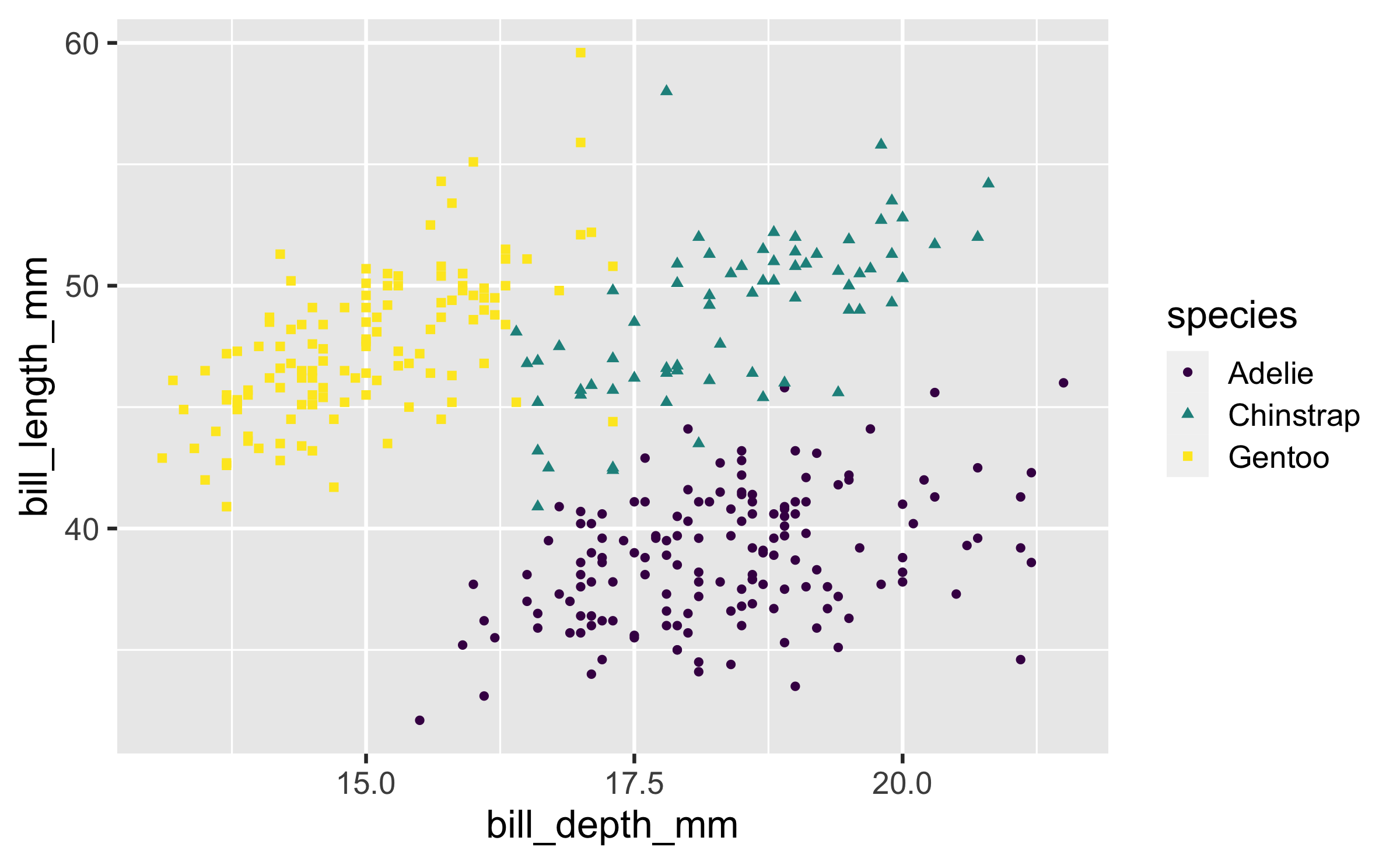
Size
ggplot(penguins, aes(x = bill_depth_mm, y = bill_length_mm, colour = species, shape = species, size = body_mass_g)) + geom_point() + scale_colour_viridis_d()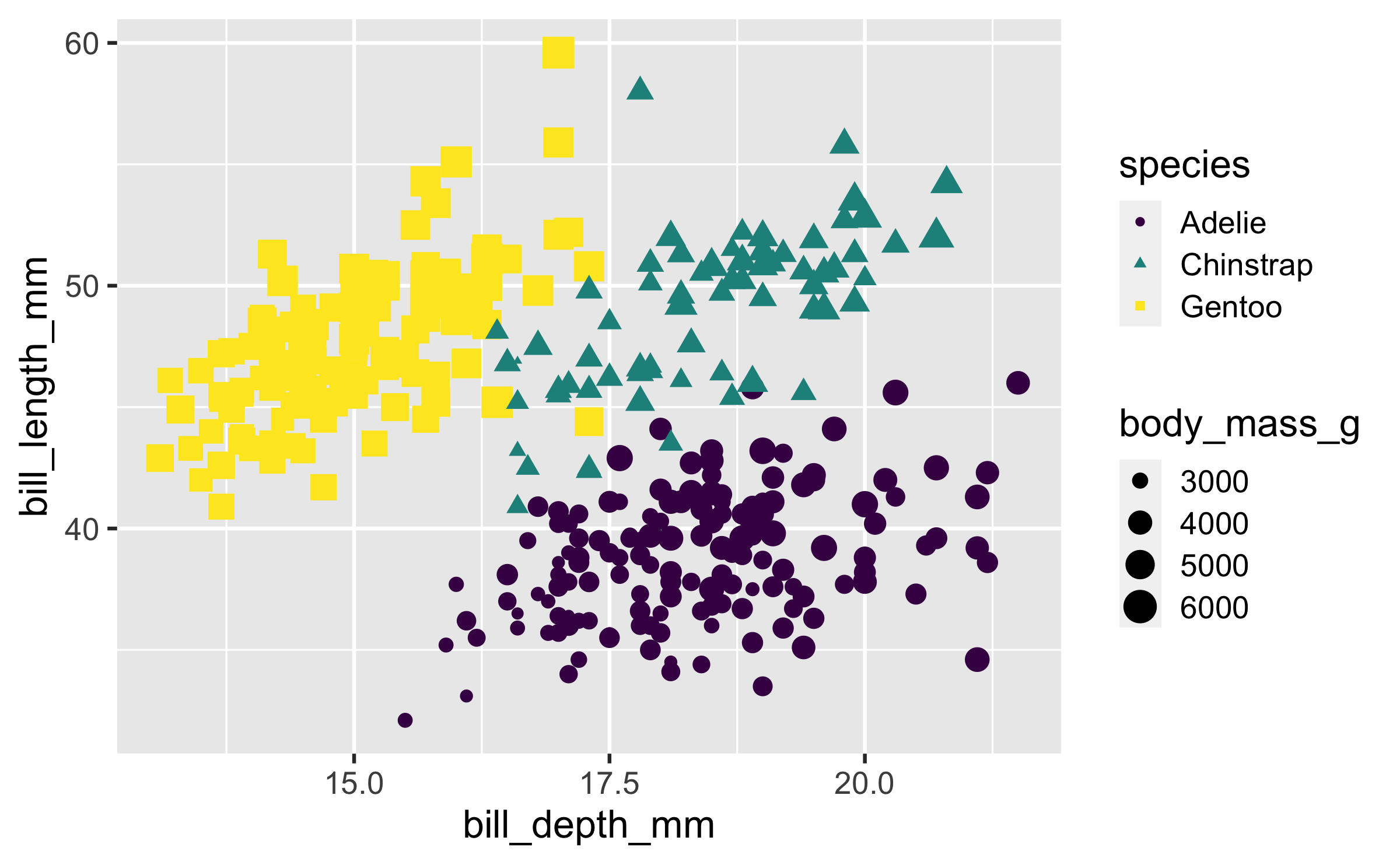
Alpha
ggplot(penguins, aes(x = bill_depth_mm, y = bill_length_mm, colour = species, shape = species, size = body_mass_g, alpha = flipper_length_mm)) + geom_point() + scale_colour_viridis_d()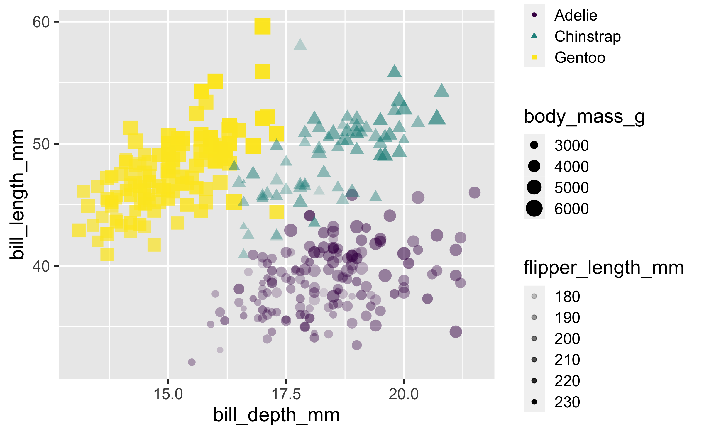
Mapping
ggplot(penguins, aes(x = bill_depth_mm, y = bill_length_mm, size = body_mass_g, alpha = flipper_length_mm)) + geom_point()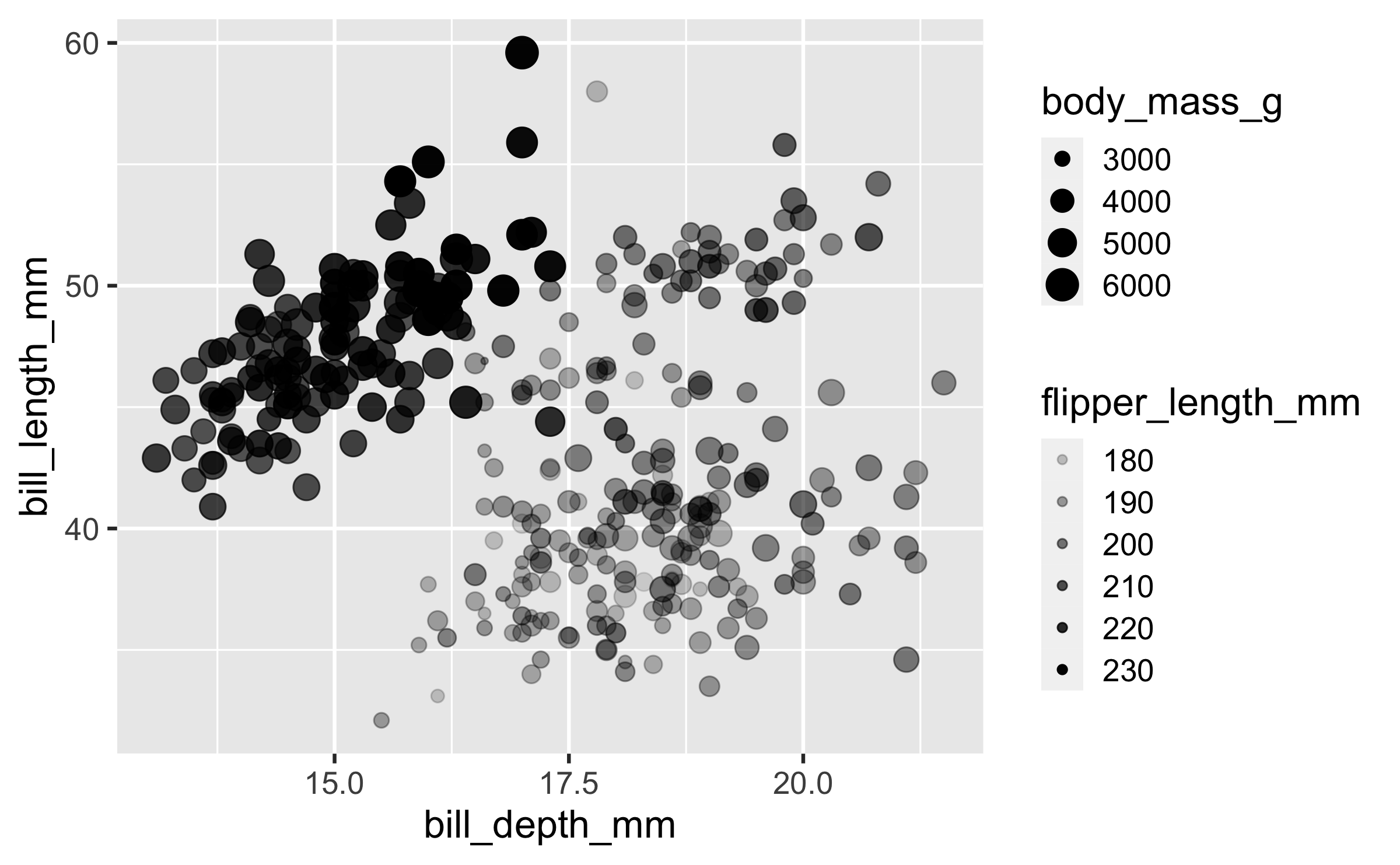
Setting
ggplot(penguins, aes(x = bill_depth_mm, y = bill_length_mm)) + geom_point(size = 2, alpha = 0.5)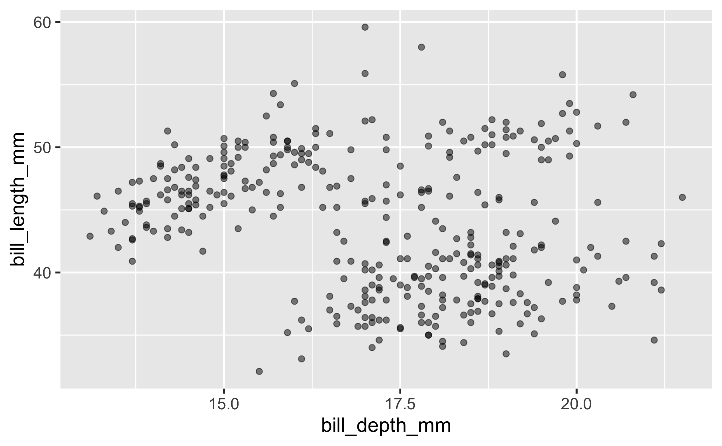
Mapping vs. setting
Mapping: Determine the size, alpha, etc. of points based on the values of a variable in the data
- goes into
aes()
- goes into
Setting: Determine the size, alpha, etc. of points not based on the values of a variable in the data
- goes into
geom_*()(this wasgeom_point()in the previous example, but we'll learn about other geoms soon!)
- goes into
Faceting
- Smaller plots that display different subsets of the data
- Useful for exploring conditional relationships and large data
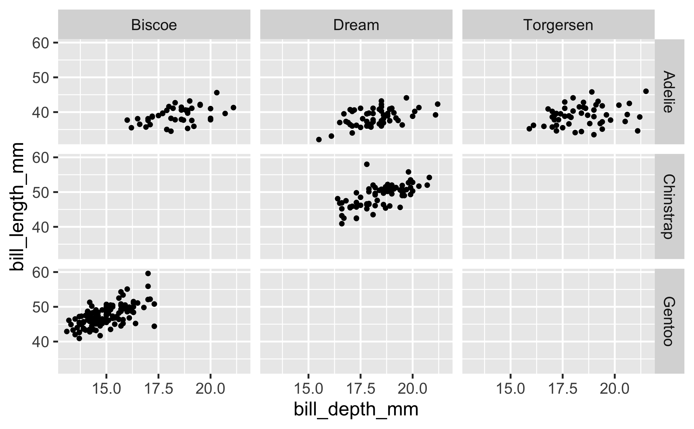
ggplot(penguins, aes(x = bill_depth_mm, y = bill_length_mm)) + geom_point() + facet_grid(species ~ island)## Warning: Removed 2 rows containing missing values (geom_point).Various ways to facet
In the next few slides describe what each plot displays. Think about how the code relates to the output.
Note: The plots in the next few slides do not have proper titles, axis labels, etc. because we want you to figure out what's happening in the plots. But you should always label your plots!
ggplot(penguins, aes(x = bill_depth_mm, y = bill_length_mm)) + geom_point() + facet_grid(species ~ sex)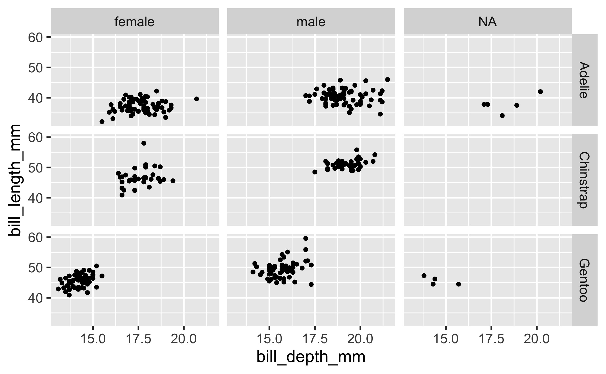
ggplot(penguins, aes(x = bill_depth_mm, y = bill_length_mm)) + geom_point() + facet_grid(sex ~ species)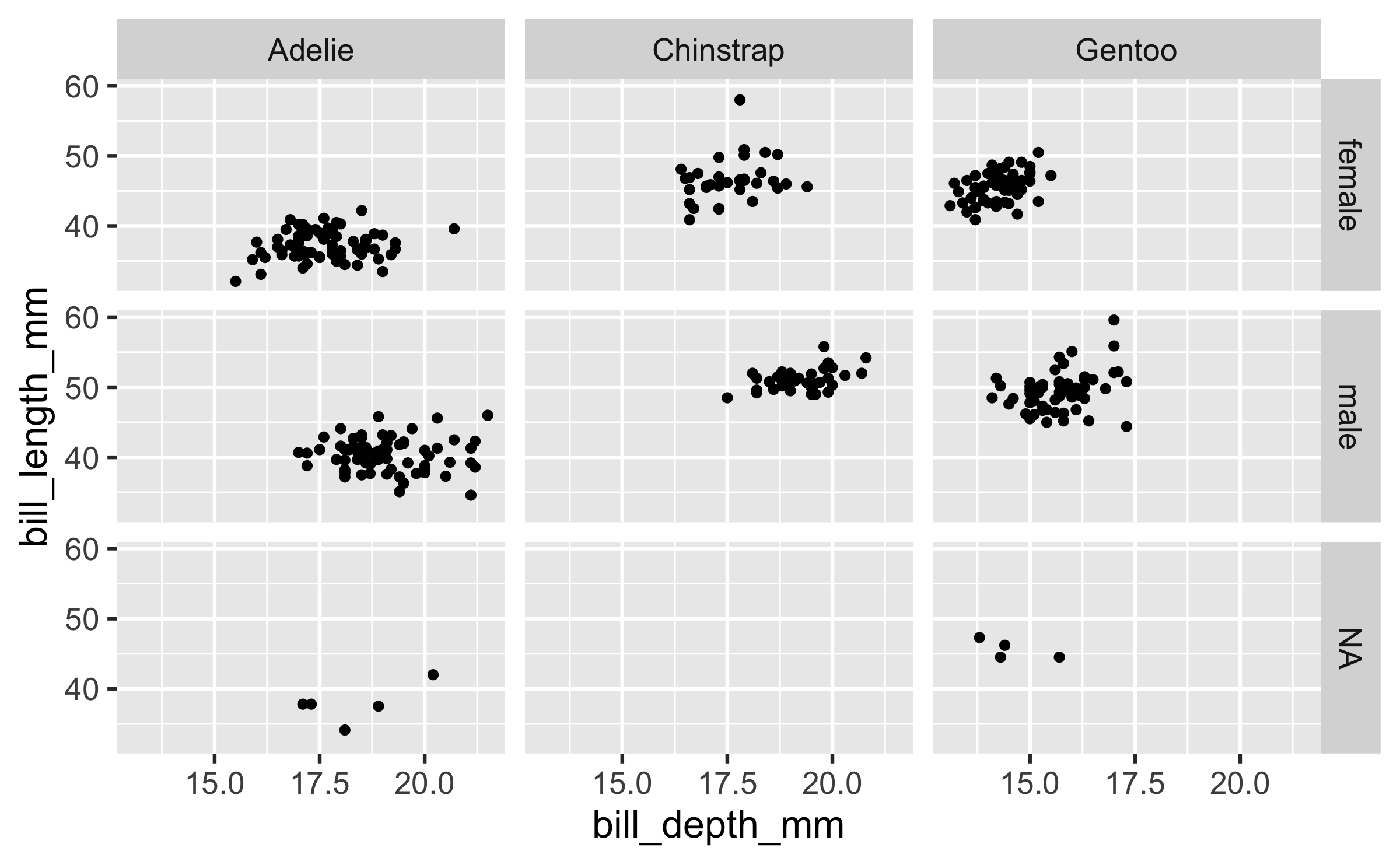
ggplot(penguins, aes(x = bill_depth_mm, y = bill_length_mm)) + geom_point() + facet_wrap(~ species)
ggplot(penguins, aes(x = bill_depth_mm, y = bill_length_mm)) + geom_point() + facet_grid(. ~ species)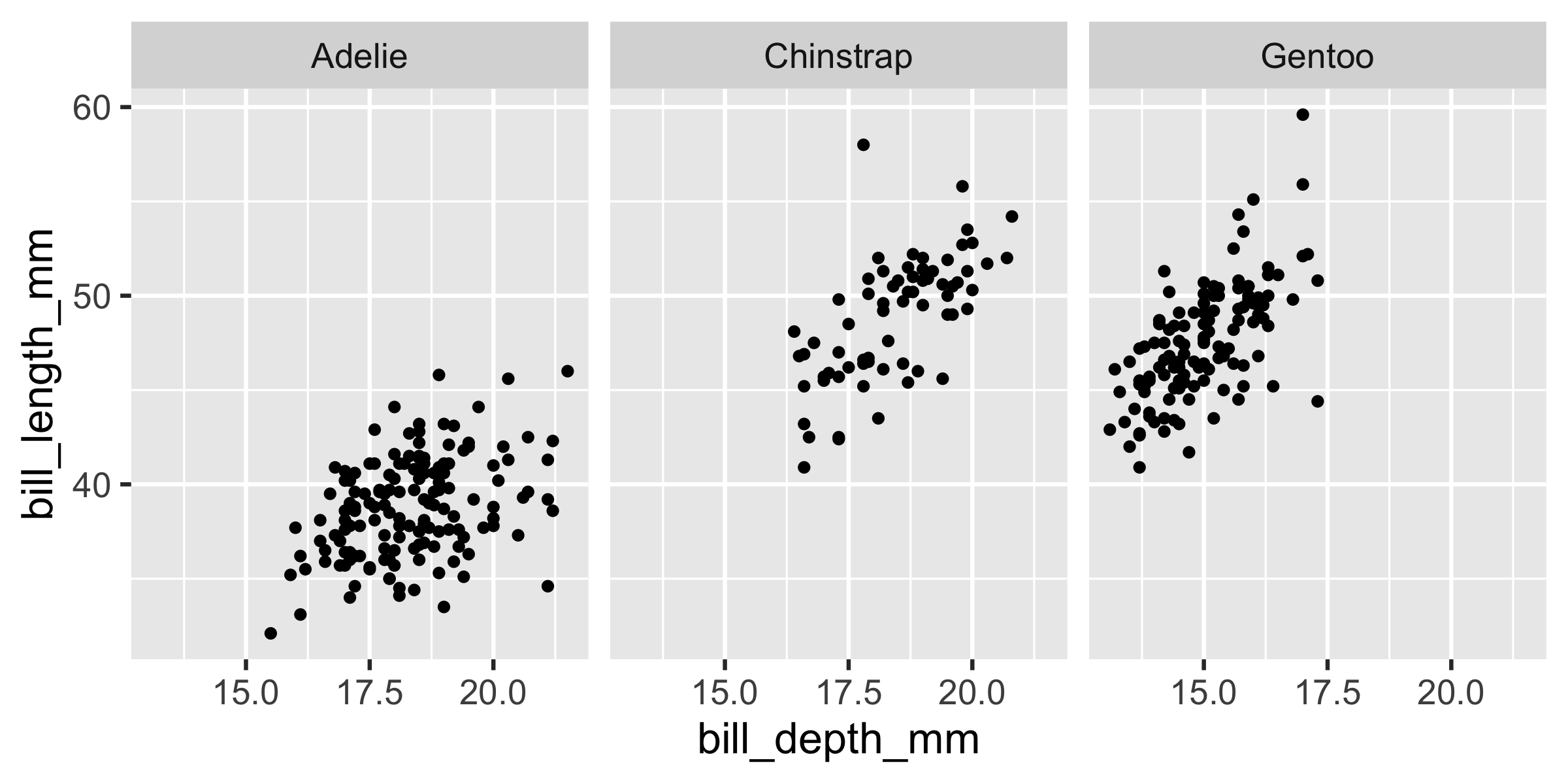
ggplot(penguins, aes(x = bill_depth_mm, y = bill_length_mm)) + geom_point() + facet_wrap(~ species, ncol = 2)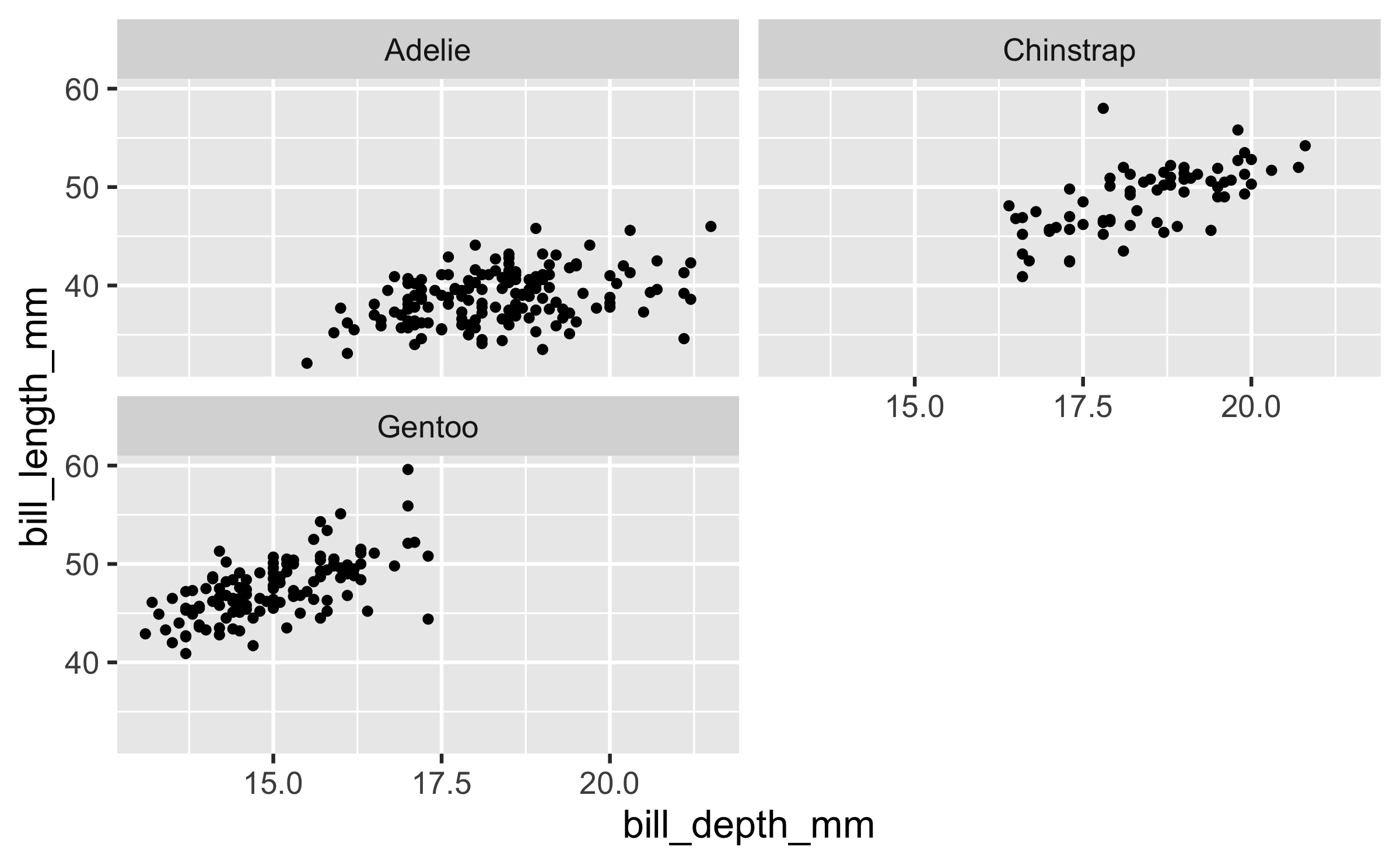
Faceting summary
facet_grid():- 2d grid
rows ~ cols- use
.for no split
facet_wrap(): 1d ribbon wrapped according to number of rows and columns specified or available plotting area
Facet and color
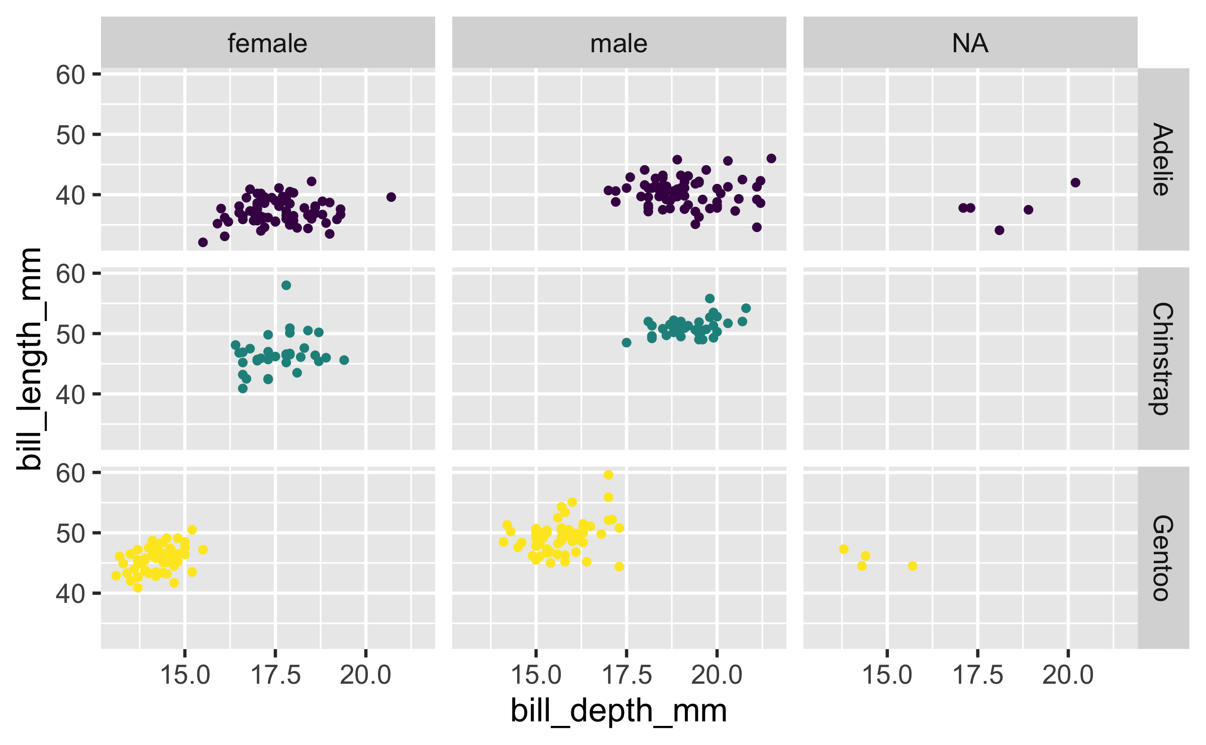
ggplot( penguins, aes(x = bill_depth_mm, y = bill_length_mm, color = species)) + geom_point() + facet_grid(species ~ sex) + scale_color_viridis_d()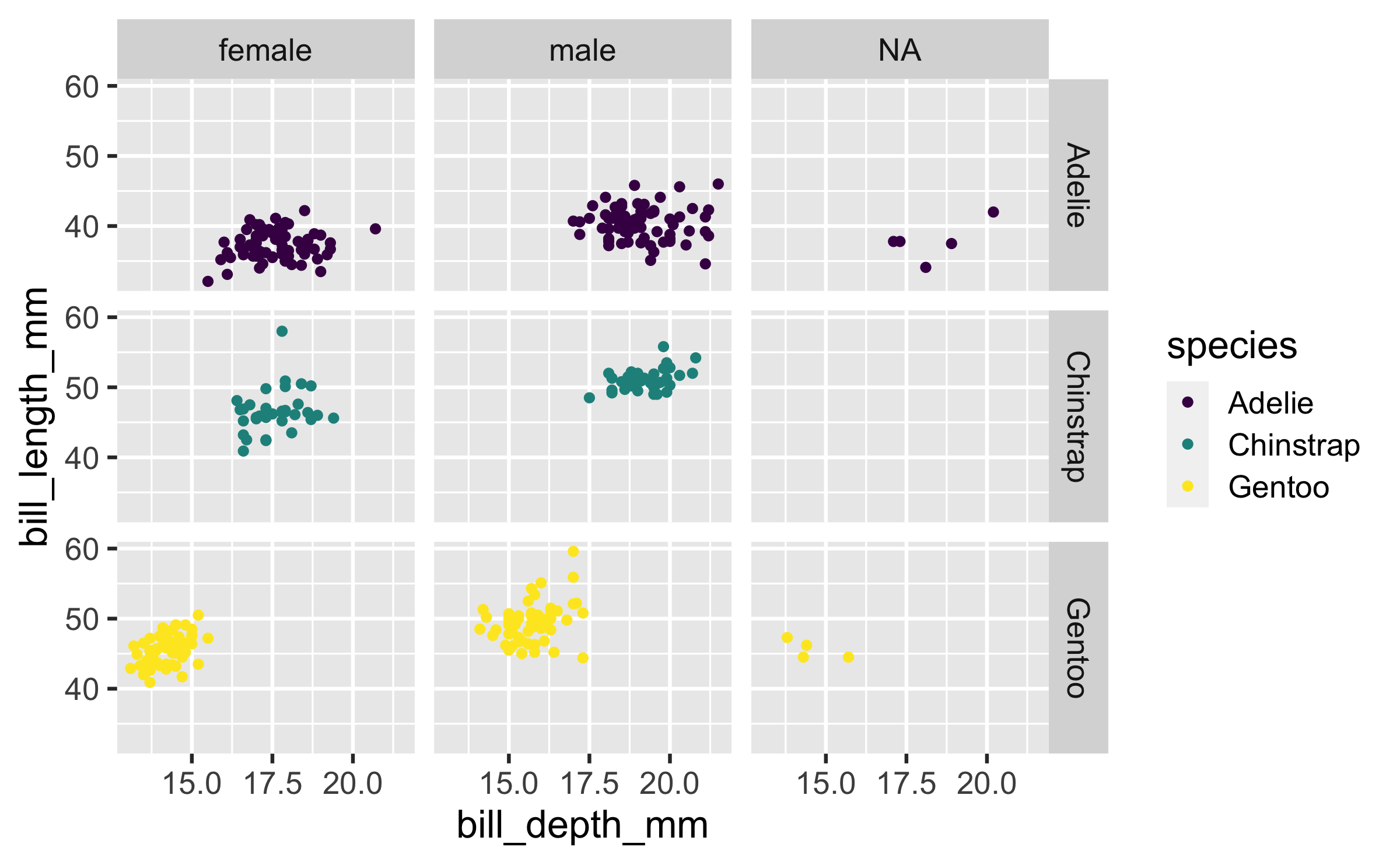
Face and color, no legend
ggplot( penguins, aes(x = bill_depth_mm, y = bill_length_mm, color = species)) + geom_point() + facet_grid(species ~ sex) + scale_color_viridis_d() + guides(color = "none")