Number of variables involved

• Univariate data analysis - distribution of single variable
• Bivariate data analysis - relationship between two variables
• Multivariate data analysis - relationship between many variables at once, usually focusing on the relationship between two while conditioning for others

Types of variables

• Numerical variables can be classified as continuous or discrete based on whether or not the variable can take on an infinite number of values or only non-negative whole numbers, respectively.
• If the variable is categorical, we can determine if it is ordinal based on whether or not the levels have a natural ordering.

Data: Lending Club

Take a peek at data

library(openintro)
glimpse(loans_full_schema)

## Rows: 10,000
## Columns: 55
## $ emp_title                        <chr> "global config enginee…
## $ emp_length                       <dbl> 3, 10, 3, 1, 10, NA, 1…
## $ state                            <fct> NJ, HI, WI, PA, CA, KY…
## $ homeownership                    <fct> MORTGAGE, RENT, RENT, …
## $ annual_income                    <dbl> 90000, 40000, 40000, 3…
## $ verified_income                  <fct> Verified, Not Verified…
## $ debt_to_income                   <dbl> 18.01, 5.04, 21.15, 10…
## $ annual_income_joint              <dbl> NA, NA, NA, NA, 57000,…
## $ verification_income_joint        <fct> , , , , Verified, , No…
## $ debt_to_income_joint             <dbl> NA, NA, NA, NA, 37.66,…
## $ delinq_2y                        <int> 0, 0, 0, 0, 0, 1, 0, 1…
## $ months_since_last_delinq         <int> 38, NA, 28, NA, NA, 3,…
## $ earliest_credit_line             <dbl> 2001, 1996, 2006, 2007…
## $ inquiries_last_12m               <int> 6, 1, 4, 0, 7, 6, 1, 1…
## $ total_credit_lines               <int> 28, 30, 31, 4, 22, 32,…
## $ open_credit_lines                <int> 10, 14, 10, 4, 16, 12,…
...

Selected variables

loans <- loans_full_schema %>%
  select(loan_amount, interest_rate, term, grade, 
         state, annual_income, homeownership, debt_to_income)
glimpse(loans)

## Rows: 10,000
## Columns: 8
## $ loan_amount    <int> 28000, 5000, 2000, 21600, 23000, 5000, 2…
## $ interest_rate  <dbl> 14.07, 12.61, 17.09, 6.72, 14.07, 6.72, …
## $ term           <dbl> 60, 36, 36, 36, 36, 36, 60, 60, 36, 36, …
## $ grade          <ord> C, C, D, A, C, A, C, B, C, A, C, B, C, B…
## $ state          <fct> NJ, HI, WI, PA, CA, KY, MI, AZ, NV, IL, …
## $ annual_income  <dbl> 90000, 40000, 40000, 30000, 35000, 34000…
## $ homeownership  <fct> MORTGAGE, RENT, RENT, RENT, RENT, OWN, M…
## $ debt_to_income <dbl> 18.01, 5.04, 21.15, 10.16, 57.96, 6.46, …

Selected variables

Variable types

Describing shapes of numerical distributions

• shape:
  • skewness: right-skewed, left-skewed, symmetric (skew is to the side of the longer tail)
  • modality: unimodal, bimodal, multimodal, uniform
• center: mean (mean), median (median), mode (not always useful)
• spread: range (range), standard deviation (sd), inter-quartile range (IQR)
• unusual observations

Histogram

ggplot(loans, aes(x = loan_amount)) +
  geom_histogram()

## `stat_bin()` using `bins = 30`. Pick better value with
## `binwidth`.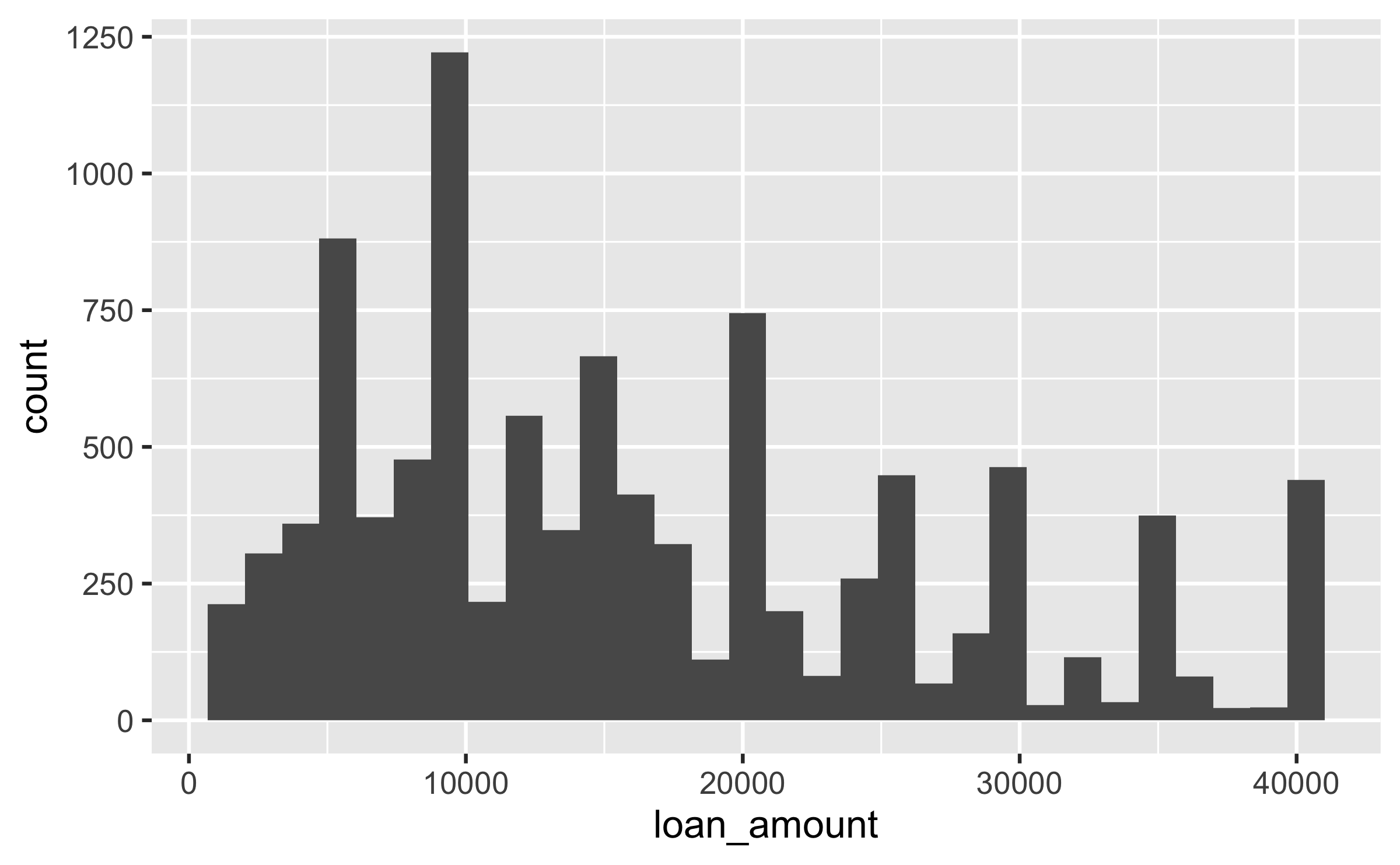

Histograms and binwidth

ggplot(loans, aes(x = loan_amount)) +
  geom_histogram(binwidth = 1000)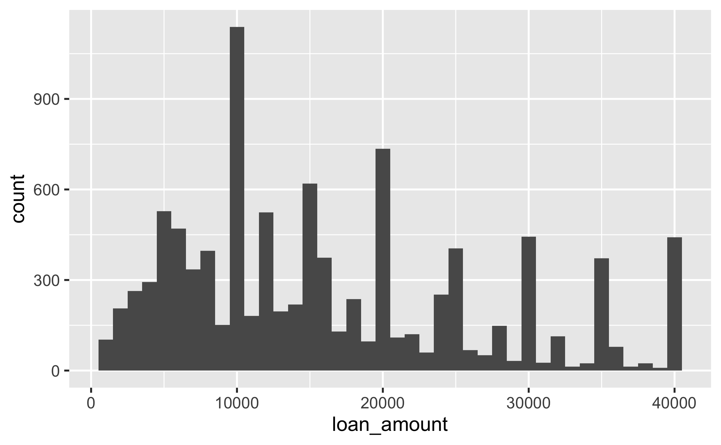

ggplot(loans, aes(x = loan_amount)) +
  geom_histogram(binwidth = 5000)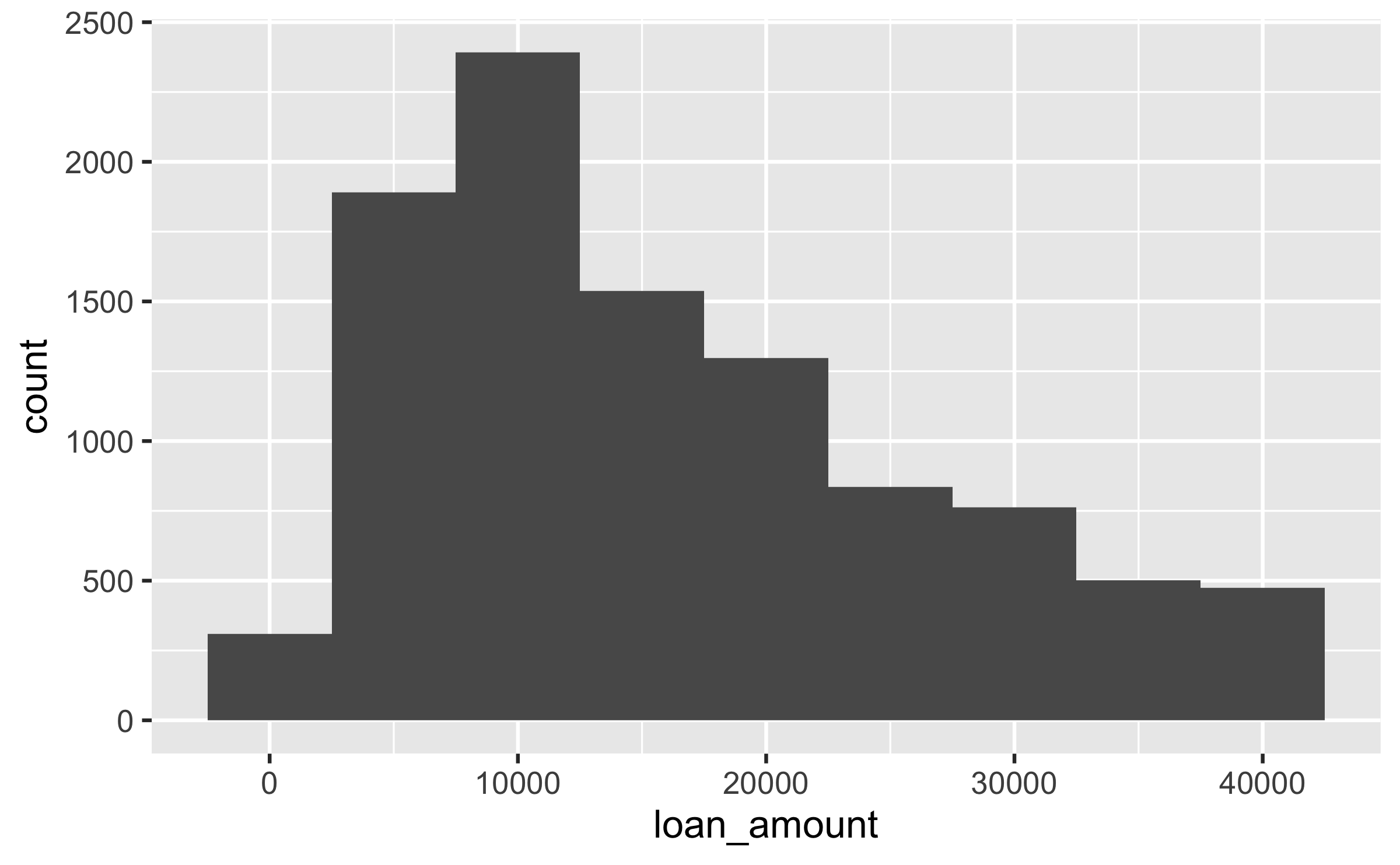

ggplot(loans, aes(x = loan_amount)) +
  geom_histogram(binwidth = 20000)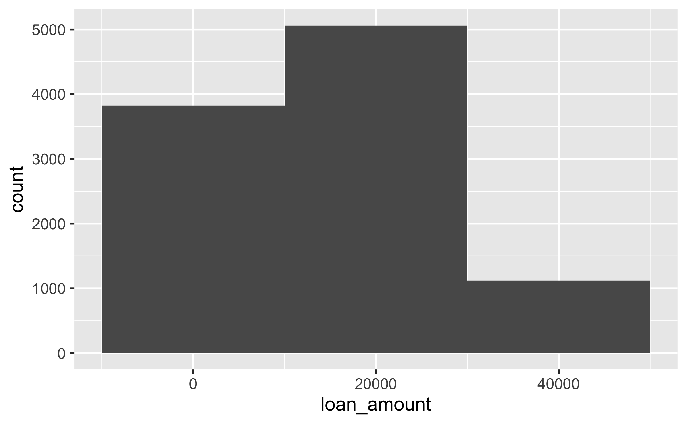

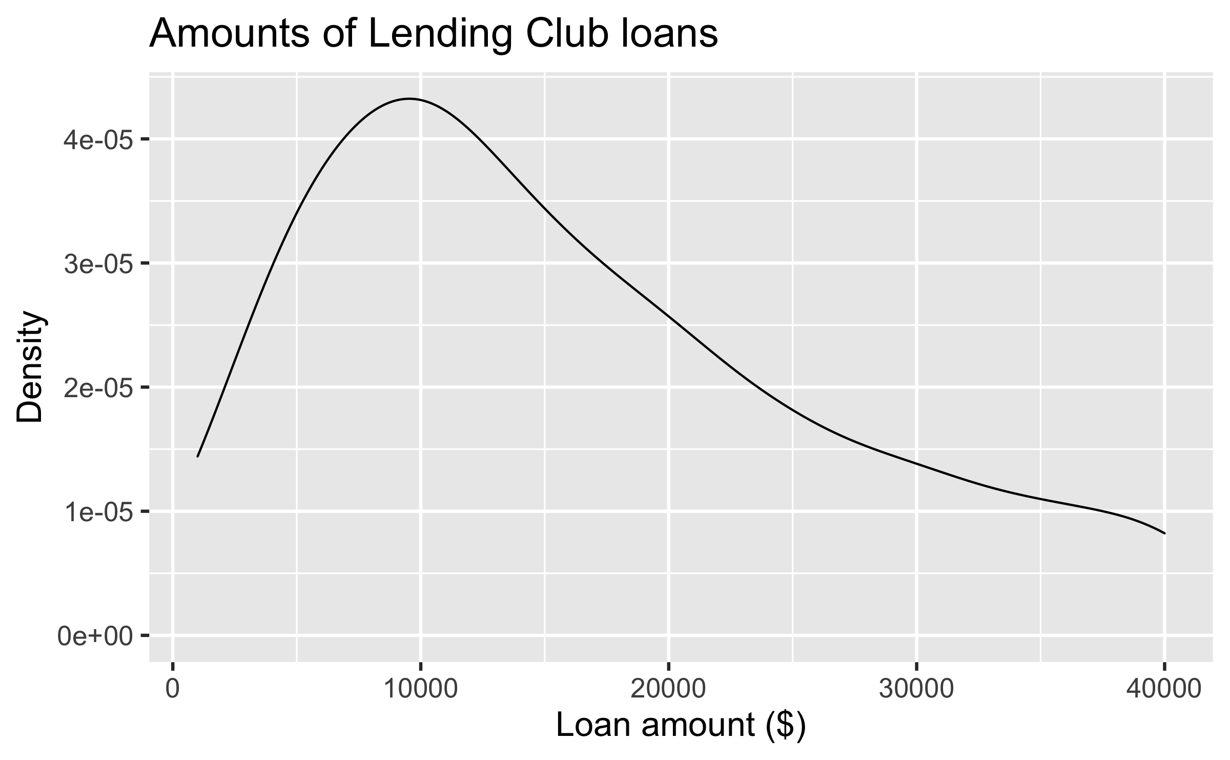
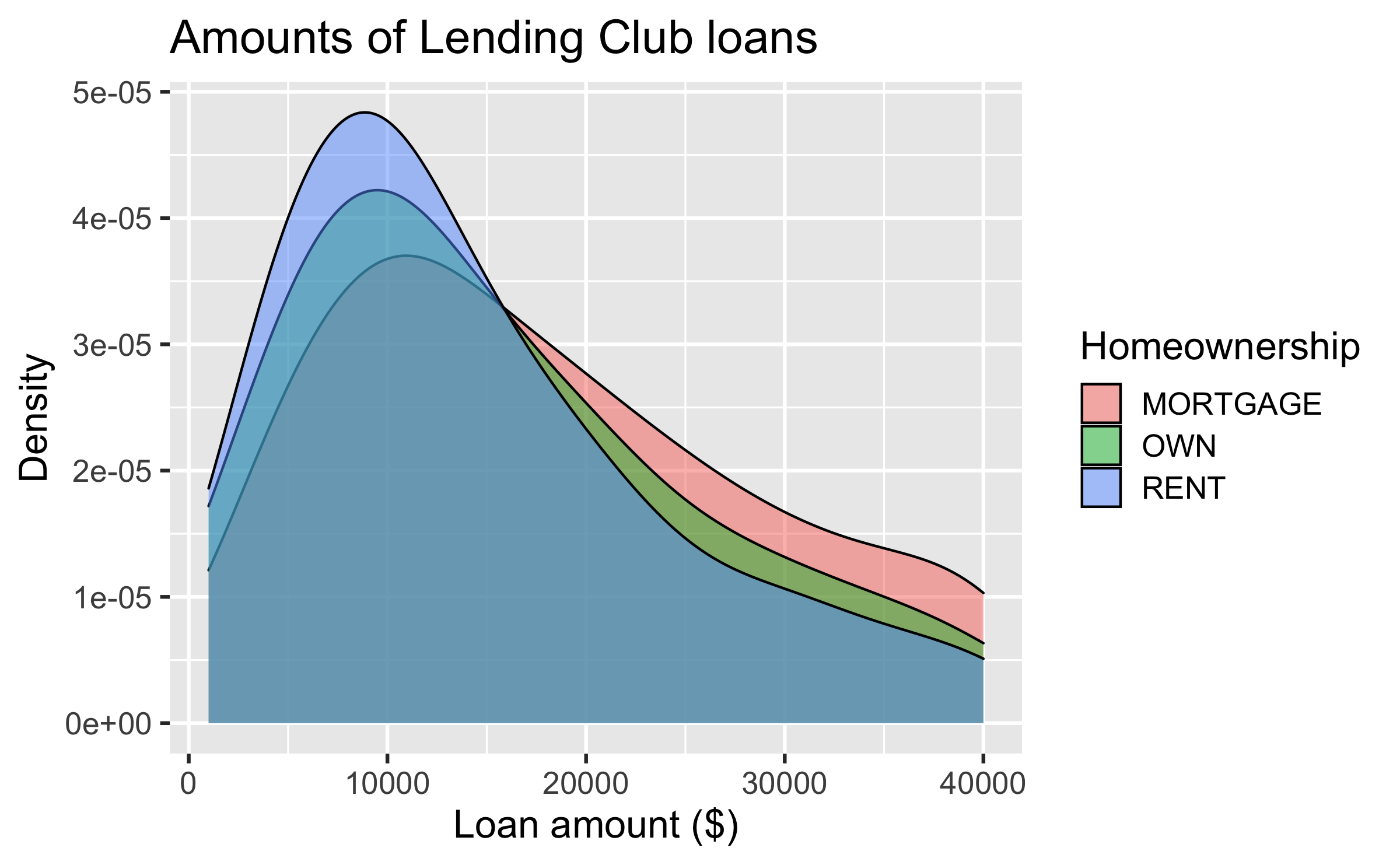
Customizing histograms

ggplot(loans, aes(x = loan_amount)) +
  geom_histogram(binwidth = 5000) +
  labs(
    x = "Loan amount ($)",
    y = "Frequency",
    title = "Amounts of Lending Club loans"
  )

Fill with a categorical variable

ggplot(loans, aes(x = loan_amount, 
                  fill = homeownership)) +
  geom_histogram(binwidth = 5000,
                 alpha = 0.5) +
  labs(
    x = "Loan amount ($)",
    y = "Frequency",
    title = "Amounts of Lending Club loans"
  )

Facet with a categorical variable

ggplot(loans, aes(x = loan_amount, fill = homeownership)) + 
  geom_histogram(binwidth = 5000) +
  labs(
    x = "Loan amount ($)",
    y = "Frequency",
    title = "Amounts of Lending Club loans"
  ) +
  facet_wrap(~ homeownership, nrow = 3)

Density plot

ggplot(loans, aes(x = loan_amount)) +
  geom_density()

Density plots and adjusting bandwidth

ggplot(loans, aes(x = loan_amount)) +
  geom_density(adjust = 0.5)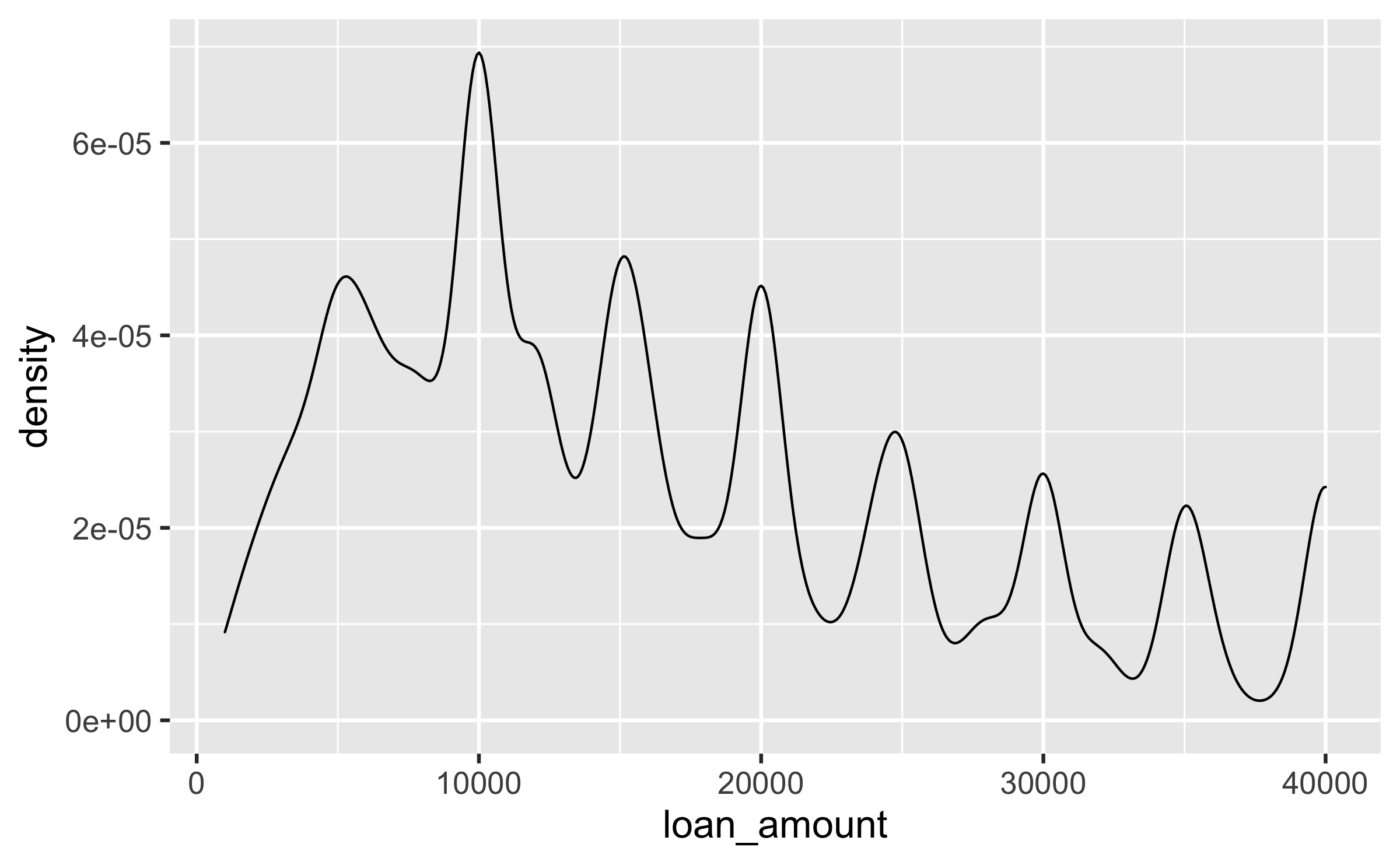

ggplot(loans, aes(x = loan_amount)) +
  geom_density(adjust = 1) # default bandwidth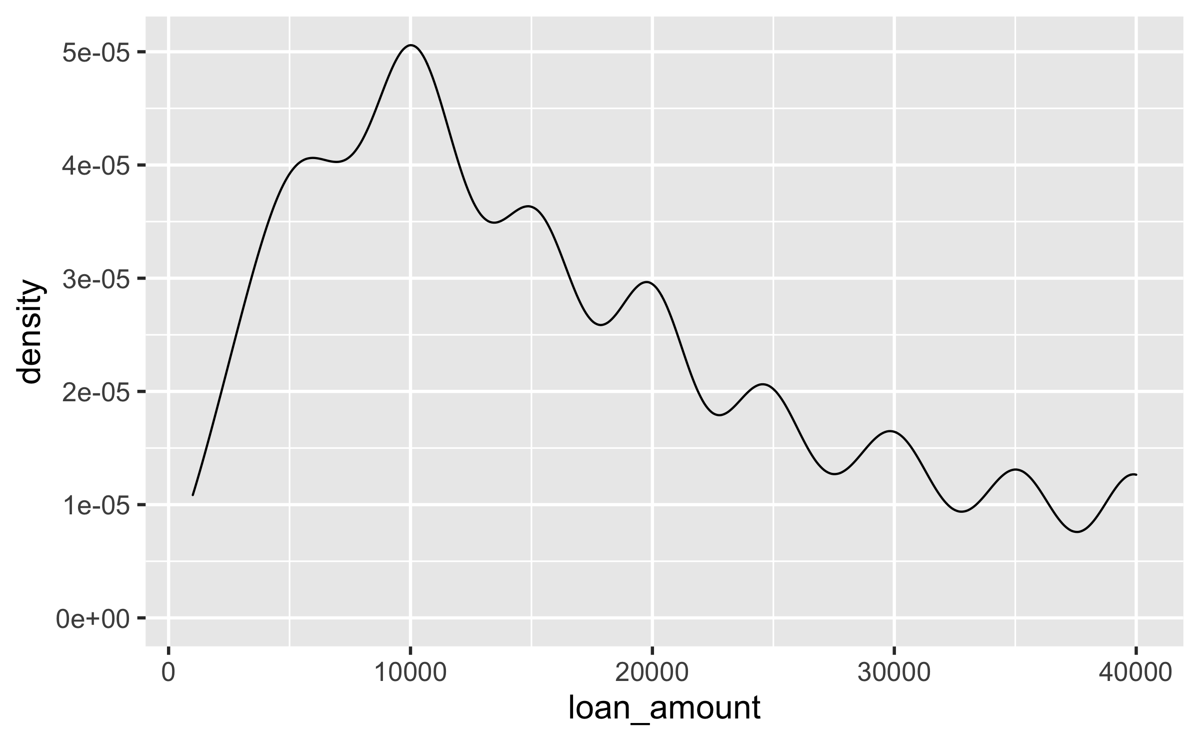

ggplot(loans, aes(x = loan_amount)) +
  geom_density(adjust = 2)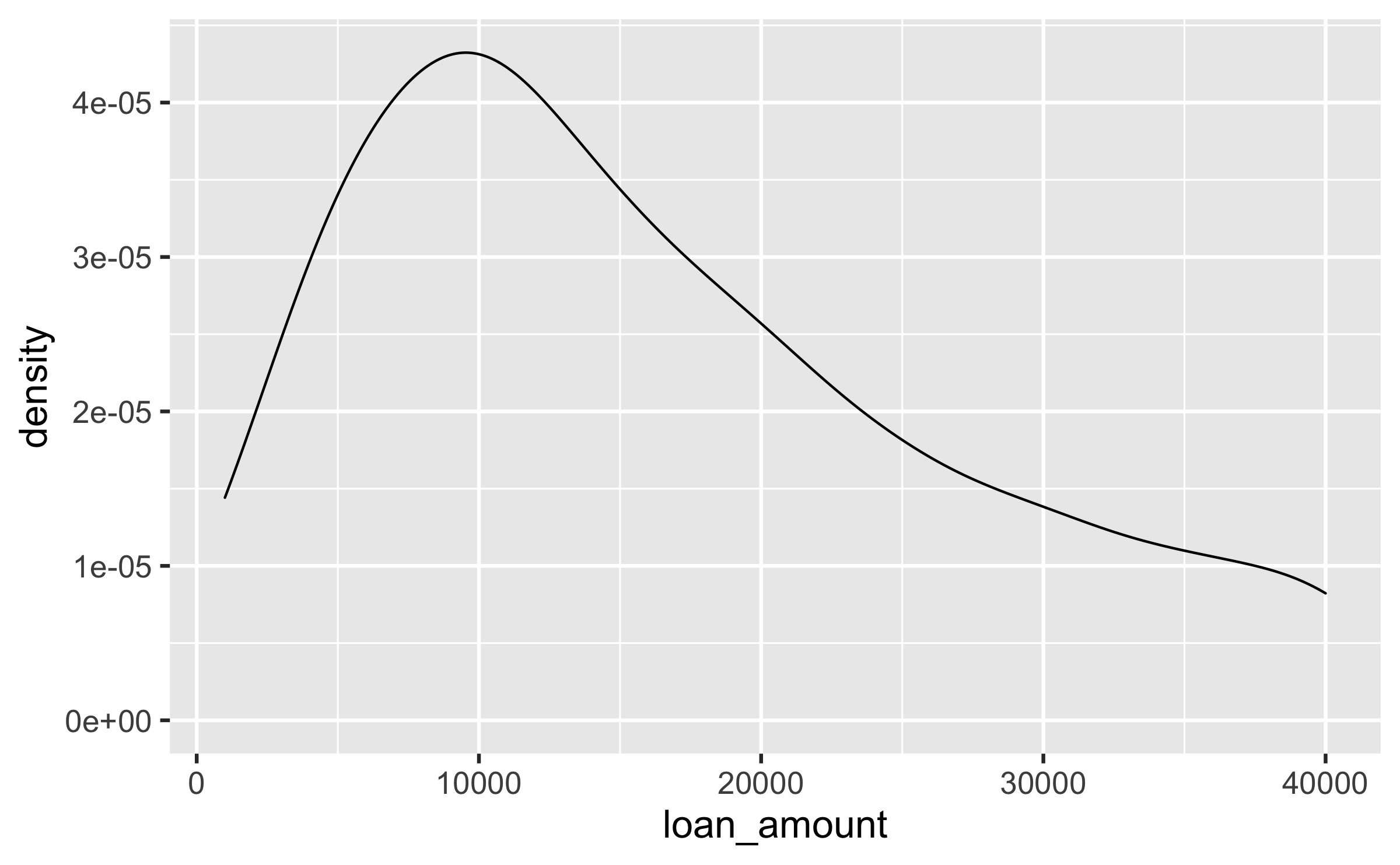

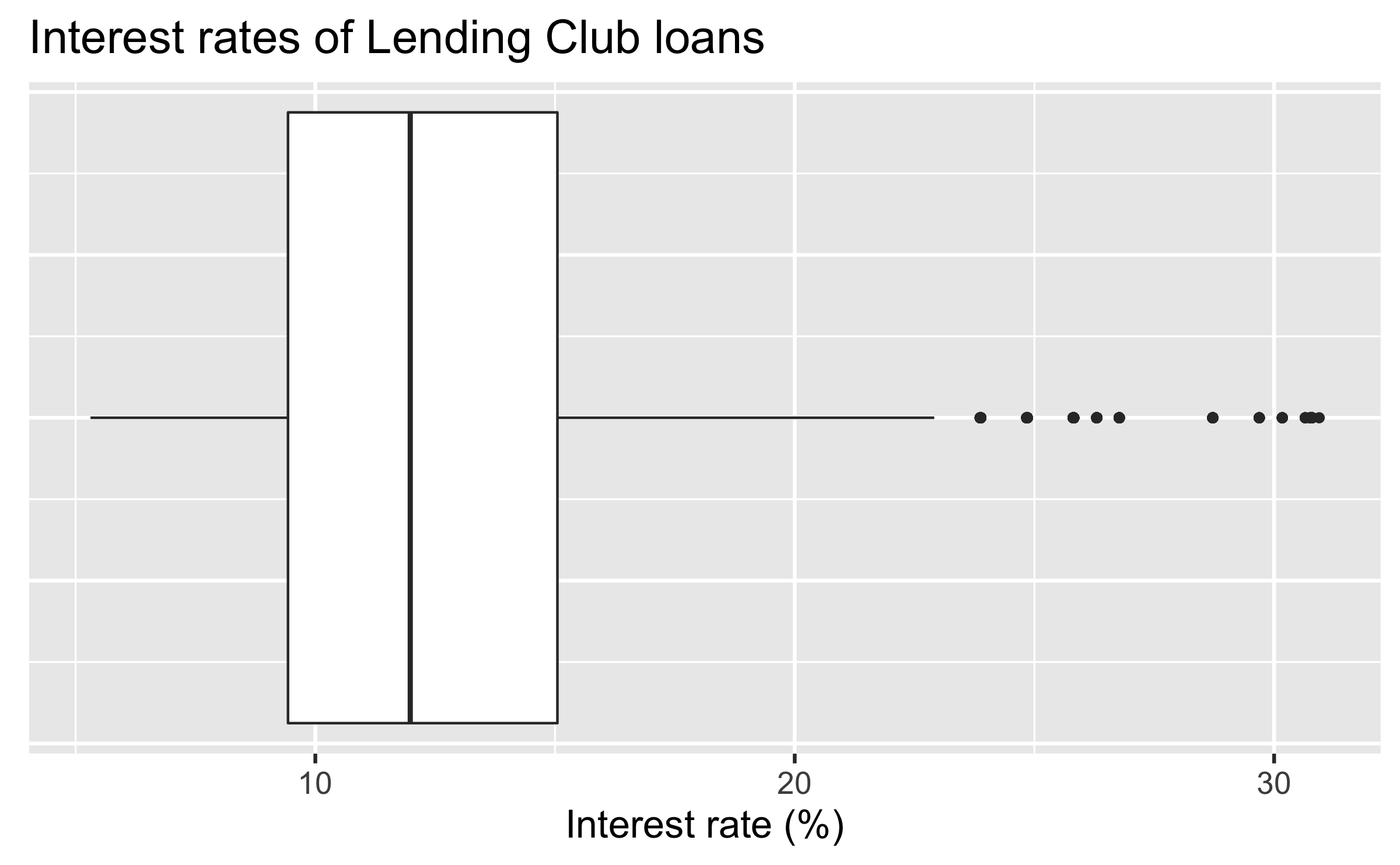
Customizing density plots

ggplot(loans, aes(x = loan_amount)) +
  geom_density(adjust = 2) +
  labs(
    x = "Loan amount ($)",
    y = "Density",
    title = "Amounts of Lending Club loans"
  )

Adding a categorical variable

ggplot(loans, aes(x = loan_amount, 
                  fill = homeownership)) +
  geom_density(adjust = 2, 
               alpha = 0.5) +
  labs(
    x = "Loan amount ($)",
    y = "Density",
    title = "Amounts of Lending Club loans", 
    fill = "Homeownership"
  )

Box plot

ggplot(loans, aes(x = interest_rate)) +
  geom_boxplot()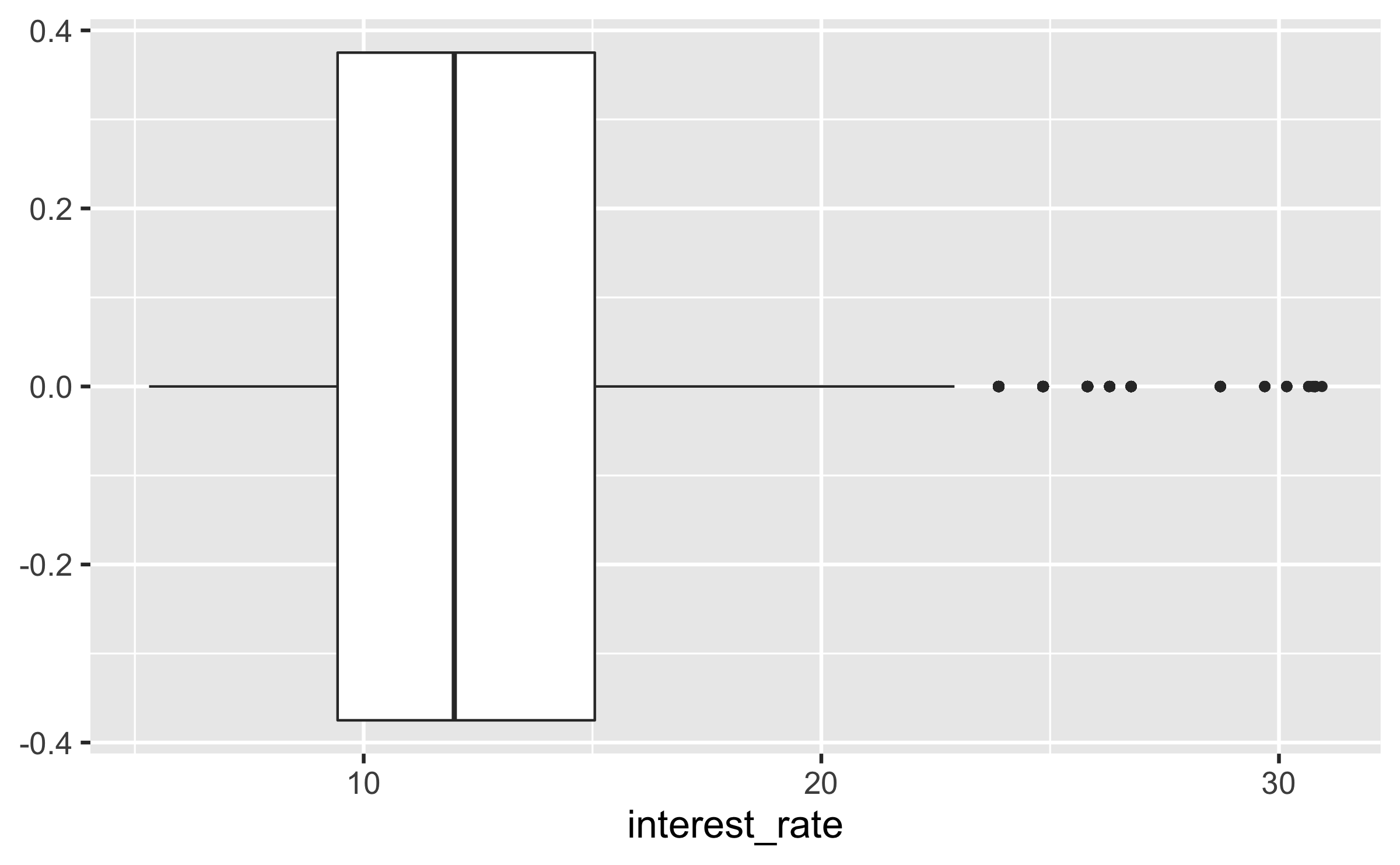

Box plot and outliers

ggplot(loans, aes(x = annual_income)) +
  geom_boxplot()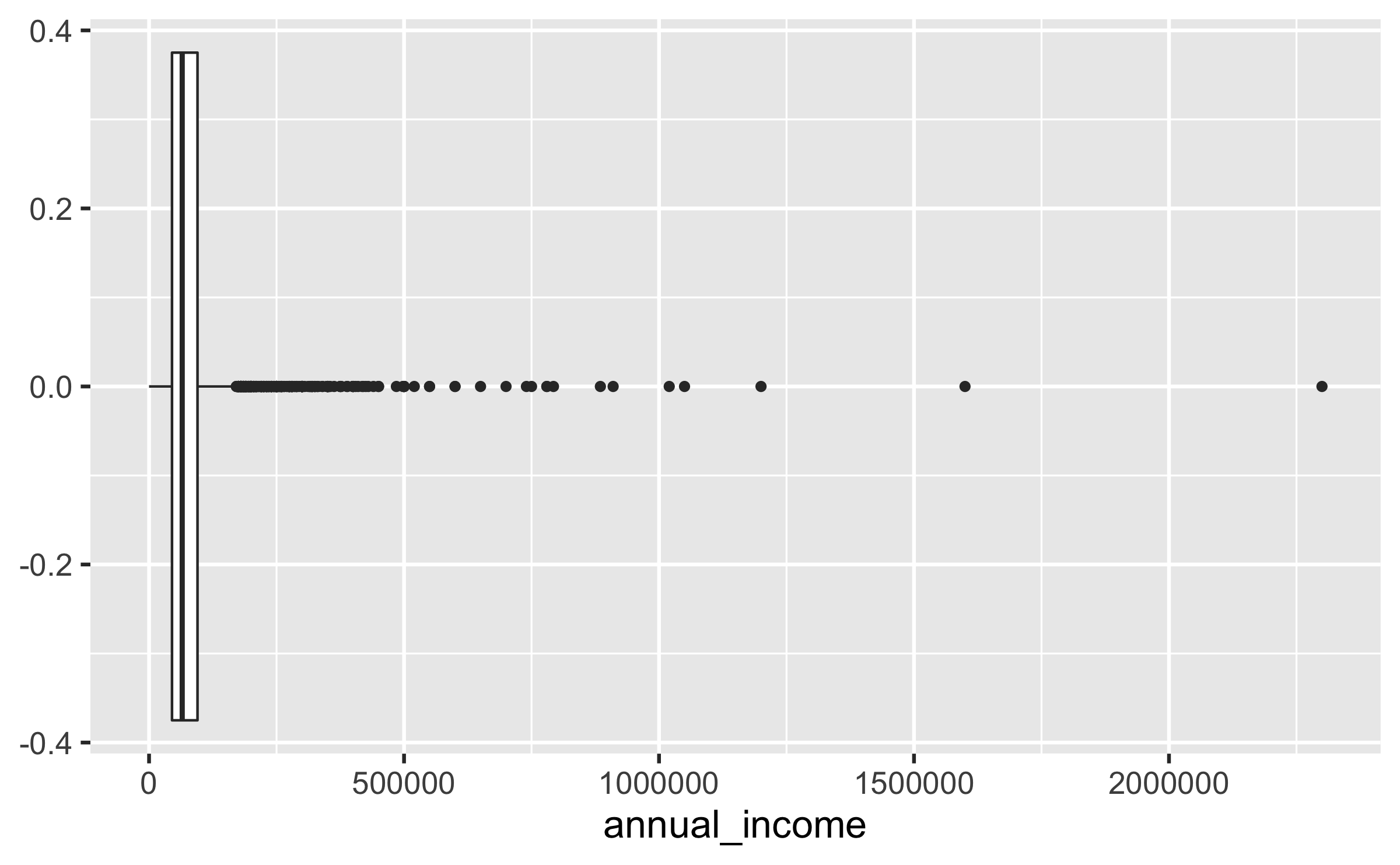

Customizing box plots

ggplot(loans, aes(x = interest_rate)) +
  geom_boxplot() +
  labs(
    x = "Interest rate (%)",
    y = NULL,
    title = "Interest rates of Lending Club loans"
  ) +
  theme(
    axis.ticks.y = element_blank(),
    axis.text.y = element_blank()
  )

Adding a categorical variable

ggplot(loans, aes(x = interest_rate,
                  y = grade)) +
  geom_boxplot() +
  labs(
    x = "Interest rate (%)",
    y = "Grade",
    title = "Interest rates of Lending Club loans",
    subtitle = "by grade of loan"
  )

Scatterplot

ggplot(loans, aes(x = debt_to_income, y = interest_rate)) +
  geom_point()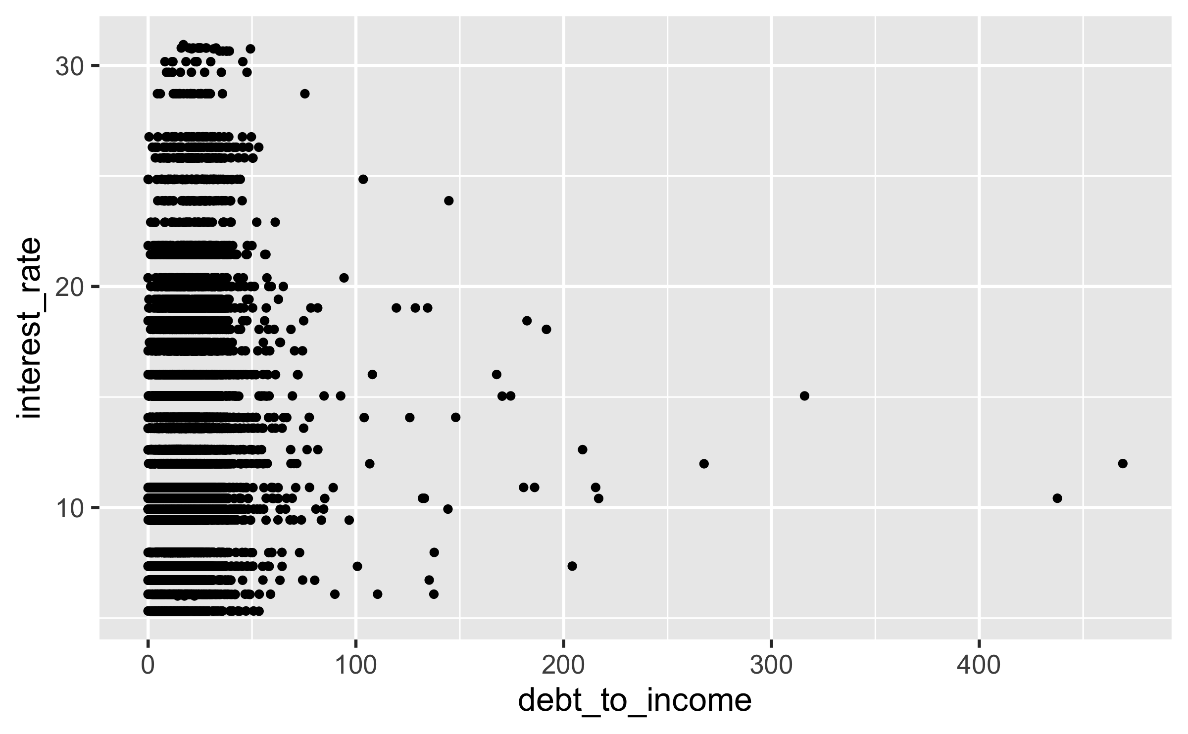

Hex plot

ggplot(loans, aes(x = debt_to_income, y = interest_rate)) +
  geom_hex()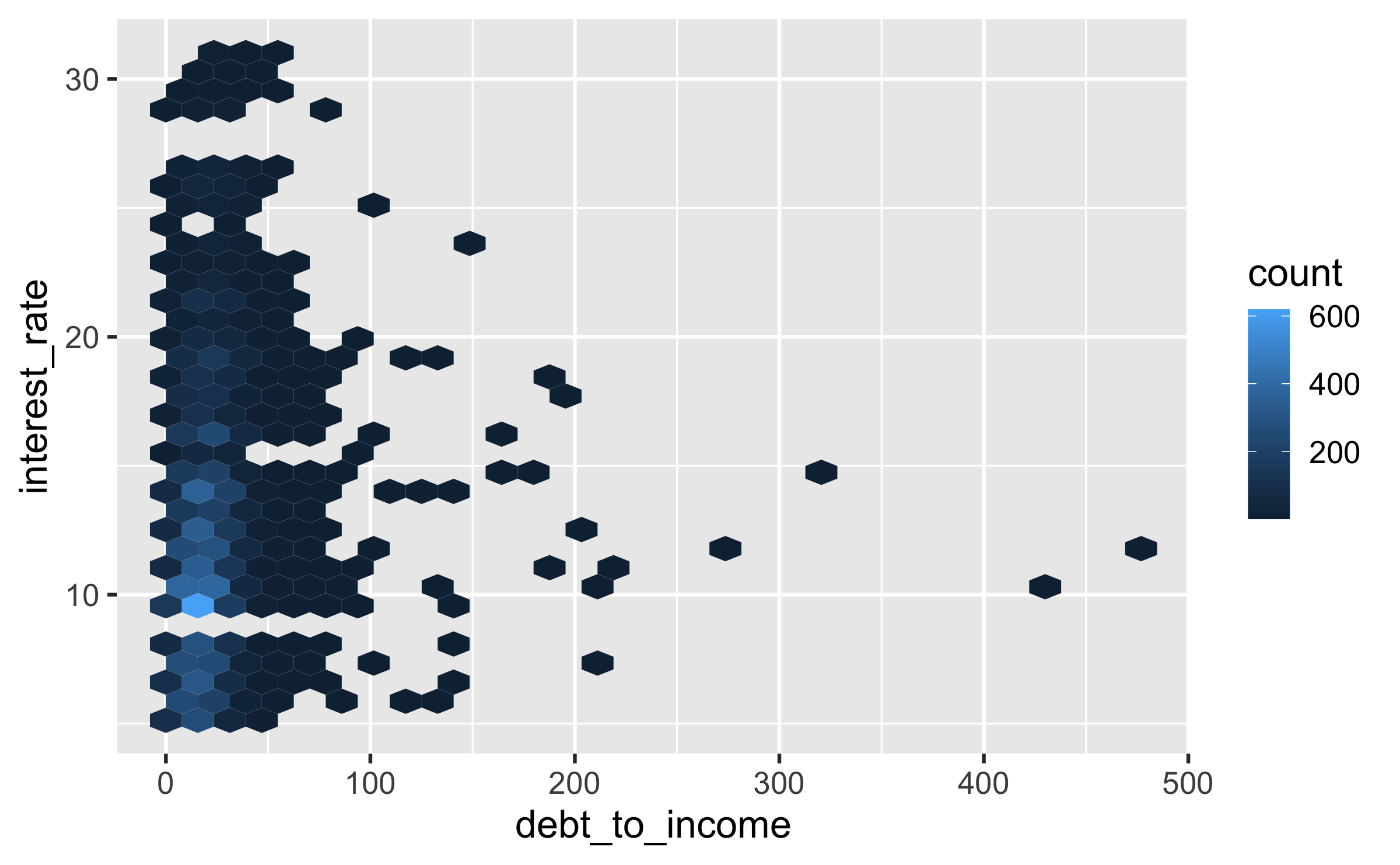

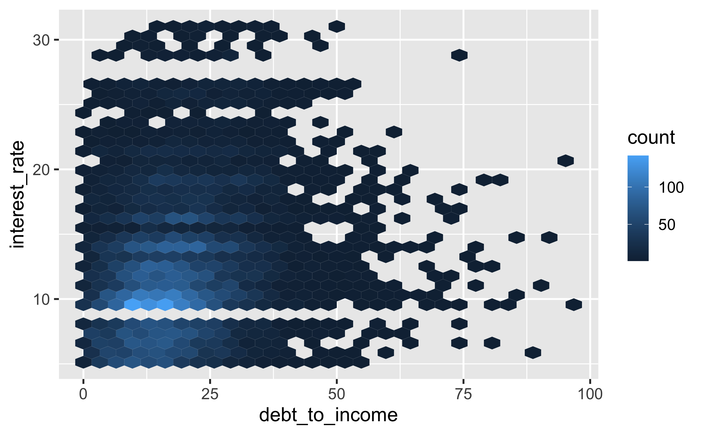
Hex plot

ggplot(loans %>% filter(debt_to_income < 100), 
       aes(x = debt_to_income, y = interest_rate)) +
  geom_hex()