+ - 0:00:00
Notes for current slide
Notes for next slide

Visualising categorical data


Data Science in a Box

1 / 15

Recap

2 / 15

Variables

  • Numerical variables can be classified as continuous or discrete based on whether or not the variable can take on an infinite number of values or only non-negative whole numbers, respectively.
  • If the variable is categorical, we can determine if it is ordinal based on whether or not the levels have a natural ordering.
3 / 15

Data

library(openintro)
loans <- loans_full_schema %>%
select(loan_amount, interest_rate, term, grade,
state, annual_income, homeownership, debt_to_income)
glimpse(loans)
## Rows: 10,000
## Columns: 8
## $ loan_amount <int> 28000, 5000, 2000, 21600, 23000, 5000, 2…
## $ interest_rate <dbl> 14.07, 12.61, 17.09, 6.72, 14.07, 6.72, …
## $ term <dbl> 60, 36, 36, 36, 36, 36, 60, 60, 36, 36, …
## $ grade <ord> C, C, D, A, C, A, C, B, C, A, C, B, C, B…
## $ state <fct> NJ, HI, WI, PA, CA, KY, MI, AZ, NV, IL, …
## $ annual_income <dbl> 90000, 40000, 40000, 30000, 35000, 34000…
## $ homeownership <fct> MORTGAGE, RENT, RENT, RENT, RENT, OWN, M…
## $ debt_to_income <dbl> 18.01, 5.04, 21.15, 10.16, 57.96, 6.46, …
4 / 15

Bar plot

5 / 15

Bar plot

ggplot(loans, aes(x = homeownership)) +
geom_bar()

6 / 15

Segmented bar plot

ggplot(loans, aes(x = homeownership,
fill = grade)) +
geom_bar()
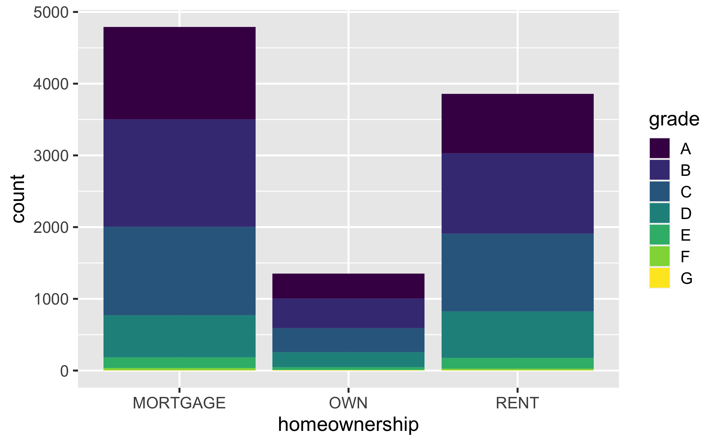
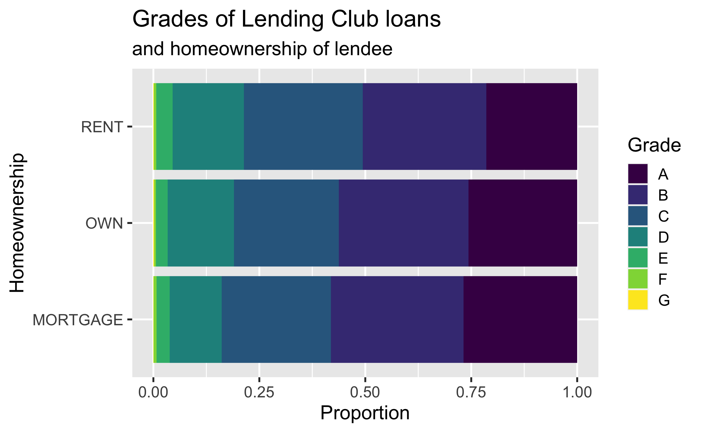
7 / 15

Segmented bar plot

ggplot(loans, aes(x = homeownership, fill = grade)) +
geom_bar(position = "fill")

8 / 15

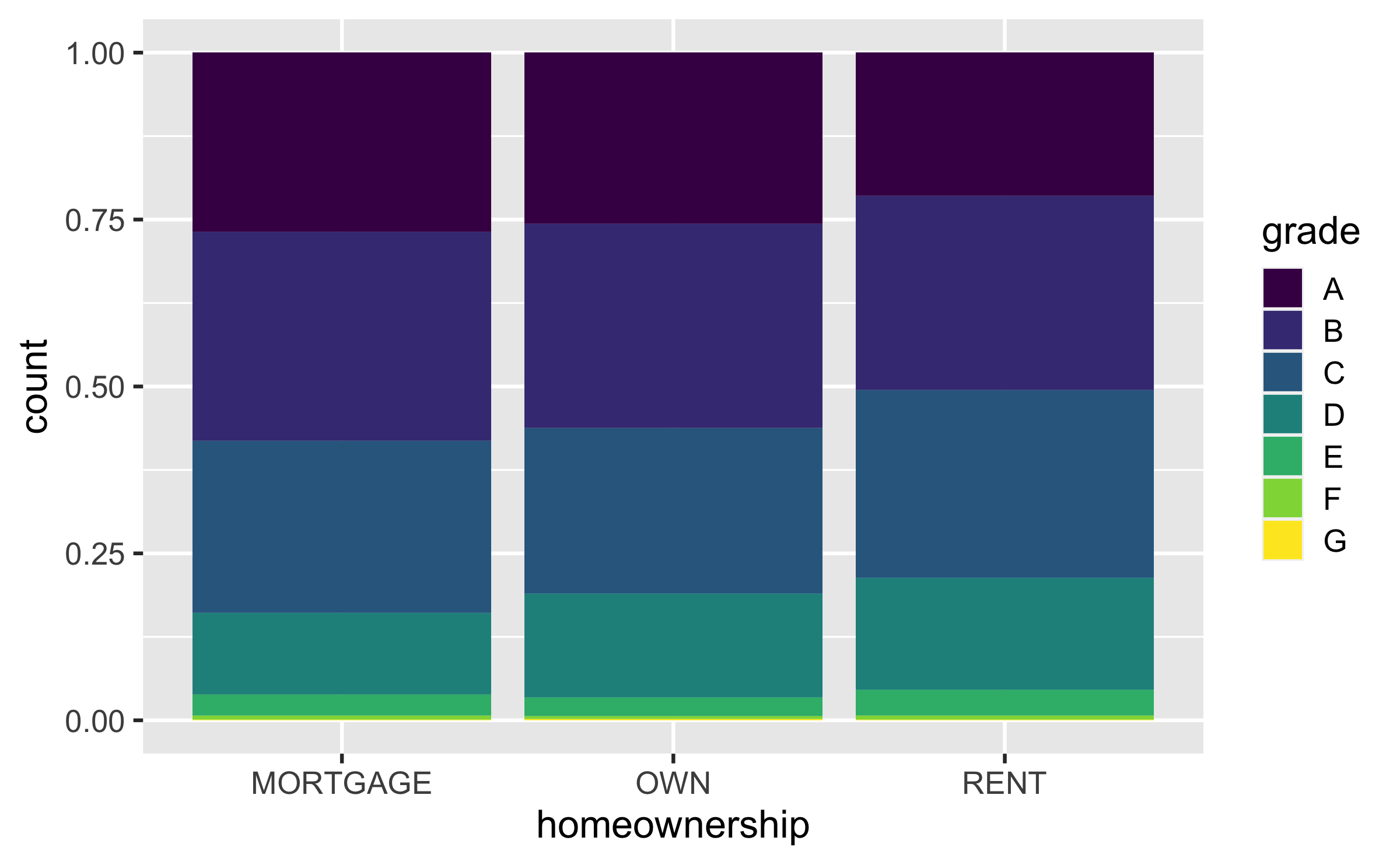
Which bar plot is a more useful representation for visualizing the relationship between homeownership and grade?

9 / 15

Customizing bar plots

ggplot(loans, aes(y = homeownership,
fill = grade)) +
geom_bar(position = "fill") +
labs(
x = "Proportion",
y = "Homeownership",
fill = "Grade",
title = "Grades of Lending Club loans",
subtitle = "and homeownership of lendee"
)
10 / 15

Relationships between numerical and categorical variables

11 / 15

Already talked about...

  • Colouring and faceting histograms and density plots
  • Side-by-side box plots
12 / 15

Violin plots

ggplot(loans, aes(x = homeownership, y = loan_amount)) +
geom_violin()
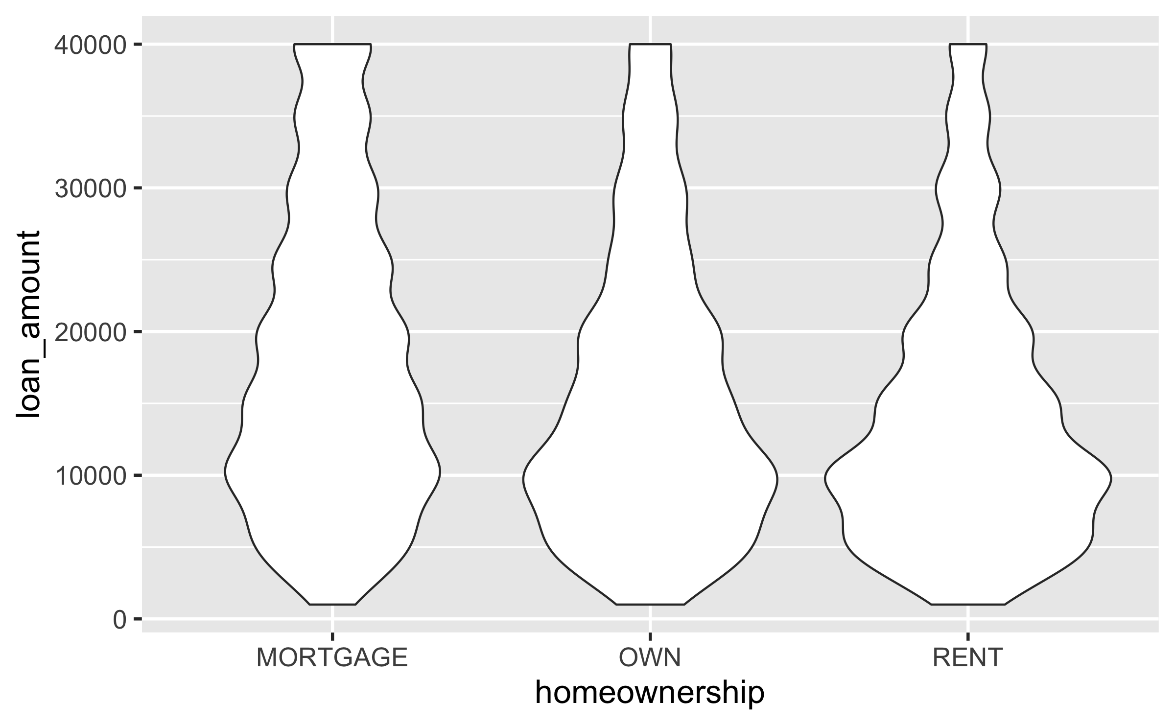
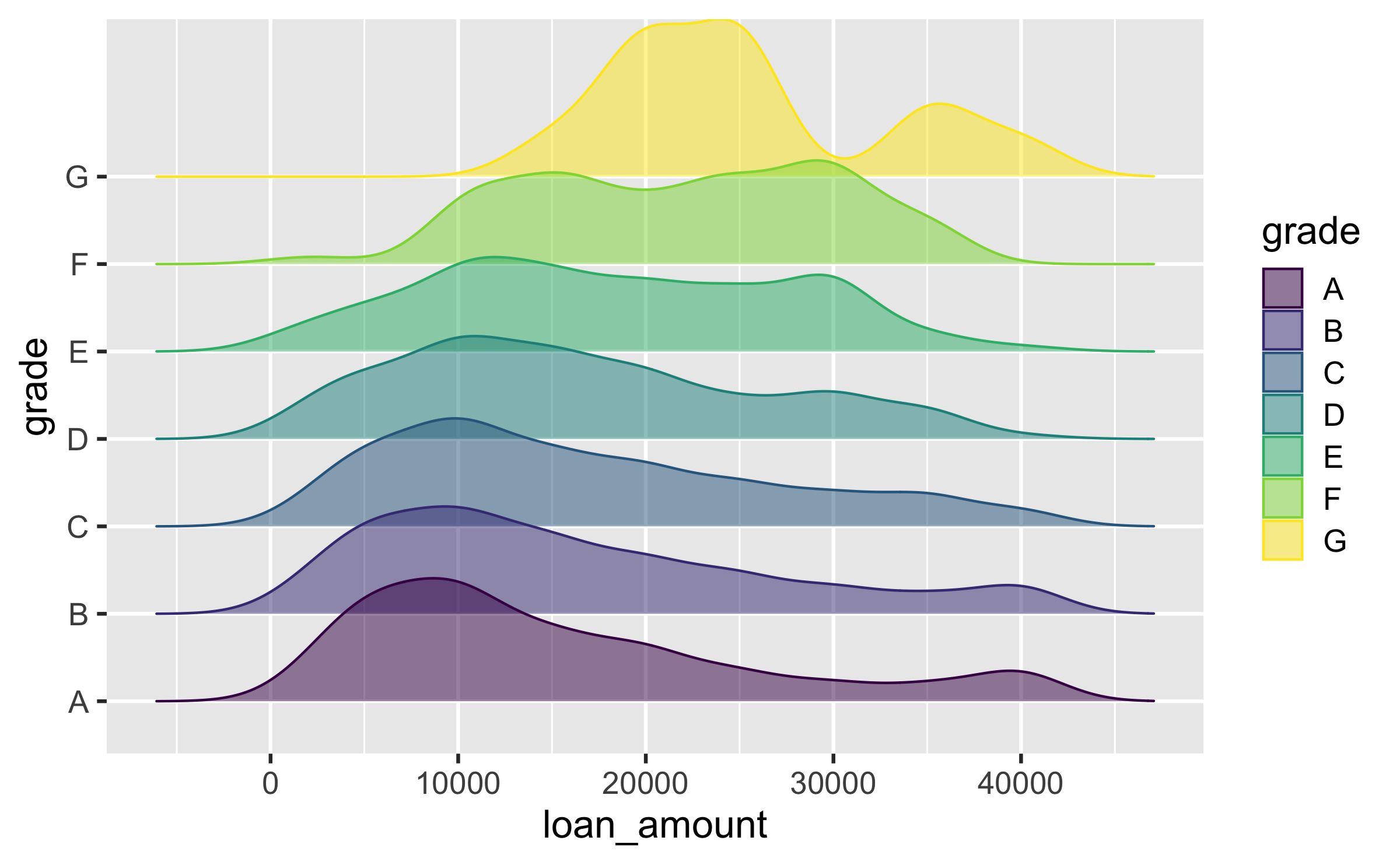
13 / 15

Ridge plots

library(ggridges)
ggplot(loans, aes(x = loan_amount, y = grade, fill = grade, color = grade)) +
geom_density_ridges(alpha = 0.5)

14 / 15

Recap

2 / 15
Paused

Help

Keyboard shortcuts

, , Pg Up, k Go to previous slide
, , Pg Dn, Space, j Go to next slide
Home Go to first slide
End Go to last slide
Number + Return Go to specific slide
b / m / f Toggle blackout / mirrored / fullscreen mode
c Clone slideshow
p Toggle presenter mode
t Restart the presentation timer
?, h Toggle this help
Esc Back to slideshow