A grammar of data wrangling...

... based on the concepts of functions as verbs that manipulate data frames

Rules of dplyr functions

• First argument is always a data frame
• Subsequent arguments say what to do with that data frame
• Always return a data frame
• Don't modify in place

Data: Hotel bookings

• Data from two hotels: one resort and one city hotel
• Observations: Each row represents a hotel booking
• Goal for original data collection: Development of prediction models to classify a hotel booking's likelihood to be cancelled (Antonia et al., 2019)

hotels <- read_csv("data/hotels.csv")

First look: Variables

names(hotels)

##  [1] "hotel"                         
##  [2] "is_canceled"                   
##  [3] "lead_time"                     
##  [4] "arrival_date_year"             
##  [5] "arrival_date_month"            
##  [6] "arrival_date_week_number"      
##  [7] "arrival_date_day_of_month"     
##  [8] "stays_in_weekend_nights"       
##  [9] "stays_in_week_nights"          
## [10] "adults"                        
## [11] "children"                      
## [12] "babies"                        
## [13] "meal"                          
## [14] "country"                       
## [15] "market_segment"                
## [16] "distribution_channel"          
## [17] "is_repeated_guest"             
## [18] "previous_cancellations"        
...

Second look: Overview

glimpse(hotels)

## Rows: 119,390
## Columns: 32
## $ hotel                          <chr> "Resort Hotel", "Resort …
## $ is_canceled                    <dbl> 0, 0, 0, 0, 0, 0, 0, 0, …
## $ lead_time                      <dbl> 342, 737, 7, 13, 14, 14,…
## $ arrival_date_year              <dbl> 2015, 2015, 2015, 2015, …
## $ arrival_date_month             <chr> "July", "July", "July", …
## $ arrival_date_week_number       <dbl> 27, 27, 27, 27, 27, 27, …
## $ arrival_date_day_of_month      <dbl> 1, 1, 1, 1, 1, 1, 1, 1, …
## $ stays_in_weekend_nights        <dbl> 0, 0, 0, 0, 0, 0, 0, 0, …
## $ stays_in_week_nights           <dbl> 0, 0, 1, 1, 2, 2, 2, 2, …
## $ adults                         <dbl> 2, 2, 1, 1, 2, 2, 2, 2, …
## $ children                       <dbl> 0, 0, 0, 0, 0, 0, 0, 0, …
## $ babies                         <dbl> 0, 0, 0, 0, 0, 0, 0, 0, …
## $ meal                           <chr> "BB", "BB", "BB", "BB", …
## $ country                        <chr> "PRT", "PRT", "GBR", "GB…
## $ market_segment                 <chr> "Direct", "Direct", "Dir…
## $ distribution_channel           <chr> "Direct", "Direct", "Dir…
...

Select a single column

View only lead_time (number of days between booking and arrival date):

select(hotels, lead_time)

## # A tibble: 119,390 × 1
##   lead_time
##       <dbl>
## 1       342
## 2       737
## 3         7
## 4        13
## 5        14
## 6        14
## # … with 119,384 more rows

Select a single column

select(
  hotels, 
  lead_time
  )

Select a single column

select( 
  hotels,
  lead_time
  )

Select a single column

select( 
  hotels, 
  lead_time
  )

Select a single column

select( 
  hotels, 
  lead_time
  )

## # A tibble: 119,390 × 1
##   lead_time
##       <dbl>
## 1       342
## 2       737
## 3         7
## 4        13
## 5        14
## 6        14
## # … with 119,384 more rows

select(hotels, lead_time)

## # A tibble: 119,390 × 1
##   lead_time
##       <dbl>
## 1       342
## 2       737
## 3         7
## 4        13
## 5        14
## 6        14
## # … with 119,384 more rows

Select multiple columns

View only the hotel type and lead_time:

select(hotels, hotel, lead_time)

## # A tibble: 119,390 × 2
##   hotel        lead_time
##   <chr>            <dbl>
## 1 Resort Hotel       342
## 2 Resort Hotel       737
## 3 Resort Hotel         7
## 4 Resort Hotel        13
## 5 Resort Hotel        14
## 6 Resort Hotel        14
## # … with 119,384 more rows

Data wrangling, step-by-step

hotels %>%
  select(hotel, lead_time)

## # A tibble: 119,390 × 2
##   hotel        lead_time
##   <chr>            <dbl>
## 1 Resort Hotel       342
## 2 Resort Hotel       737
## 3 Resort Hotel         7
## 4 Resort Hotel        13
## 5 Resort Hotel        14
## 6 Resort Hotel        14
## # … with 119,384 more rows

hotels %>%
  select(hotel, lead_time) %>%
  arrange(desc(lead_time))

## # A tibble: 119,390 × 2
##   hotel        lead_time
##   <chr>            <dbl>
## 1 Resort Hotel       737
## 2 Resort Hotel       709
## 3 City Hotel         629
## 4 City Hotel         629
## 5 City Hotel         629
## 6 City Hotel         629
## # … with 119,384 more rows

What is a pipe?

In programming, a pipe is a technique for passing information from one process to another.

hotels %>%
  select(hotel, lead_time) %>%
  arrange(desc(lead_time))

## # A tibble: 119,390 × 2
##   hotel        lead_time
##   <chr>            <dbl>
## 1 Resort Hotel       737
## 2 Resort Hotel       709
## 3 City Hotel         629
## 4 City Hotel         629
## 5 City Hotel         629
## 6 City Hotel         629
## # … with 119,384 more rows

What is a pipe?

In programming, a pipe is a technique for passing information from one process to another.

hotels %>%
  select(hotel, lead_time) %>%
  arrange(desc(lead_time))

## # A tibble: 119,390 × 2
##   hotel        lead_time
##   <chr>            <dbl>
## 1 Resort Hotel       737
## 2 Resort Hotel       709
## 3 City Hotel         629
## 4 City Hotel         629
## 5 City Hotel         629
## 6 City Hotel         629
## # … with 119,384 more rows

What is a pipe?

In programming, a pipe is a technique for passing information from one process to another.

hotels %>%
  select(hotel, lead_time) %>% 
  arrange(desc(lead_time))

## # A tibble: 119,390 × 2
##   hotel        lead_time
##   <chr>            <dbl>
## 1 Resort Hotel       737
## 2 Resort Hotel       709
## 3 City Hotel         629
## 4 City Hotel         629
## 5 City Hotel         629
## 6 City Hotel         629
## # … with 119,384 more rows

Aside

The pipe operator is implemented in the package magrittr, though we don't need to load this package explicitly since tidyverse does this for us.

How does a pipe work?

• You can think about the following sequence of actions - find keys, unlock car, start car, drive to work, park.
• Expressed as a set of nested functions in R pseudocode this would look like:

park(drive(start_car(find("keys")), to = "work"))

• Writing it out using pipes give it a more natural (and easier to read) structure:

find("keys") %>%
  start_car() %>%
  drive(to = "work") %>%
  park()

A note on piping and layering

• %>% used mainly in dplyr pipelines, we pipe the output of the previous line of code as the first input of the next line of code
• + used in ggplot2 plots is used for "layering", we create the plot in layers, separated by +

dplyr

hotels +
  select(hotel, lead_time)

## Error in select(hotel, lead_time): object 'hotel' not found

hotels %>%
  select(hotel, lead_time)

## # A tibble: 119,390 × 2
##   hotel        lead_time
##   <chr>            <dbl>
## 1 Resort Hotel       342
## 2 Resort Hotel       737
## 3 Resort Hotel         7
...

ggplot2

ggplot(hotels, aes(x = hotel, fill = deposit_type)) %>%
  geom_bar()

## Error in `validate_mapping()`:
## ! `mapping` must be created by `aes()`
## Did you use %>% instead of +?

ggplot(hotels, aes(x = hotel, fill = deposit_type)) +
  geom_bar()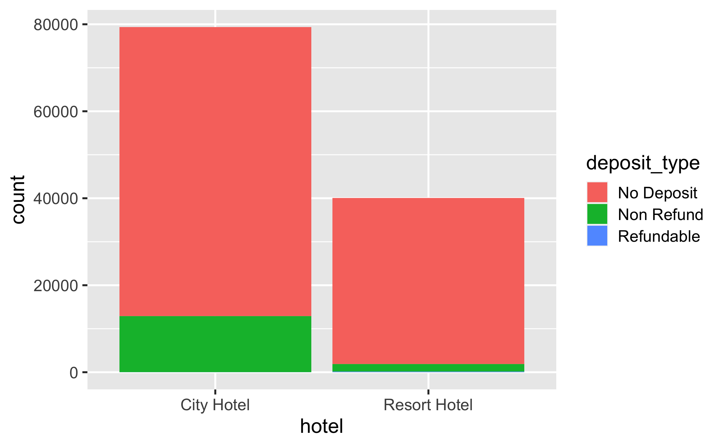

Code styling

Many of the styling principles are consistent across %>% and +:

• always a space before
• always a line break after (for pipelines with more than 2 lines)

❌

ggplot(hotels,aes(x=hotel,y=deposit_type))+geom_bar()

✅

ggplot(hotels, aes(x = hotel, y = deposit_type)) + 
  geom_bar()