Importing data

Data Science in a Box

datasciencebox.org

1 / 32

Reading rectangular data into R

2 / 32

3 / 32

readr

read_csv() - comma delimited files
read_csv2() - semicolon separated files (common in countries where , is used as the decimal place)
read_tsv() - tab delimited files
read_delim() - reads in files with any delimiter
read_fwf() - fixed width files
...

4 / 32

readr

read_csv() - comma delimited files
read_csv2() - semicolon separated files (common in countries where , is used as the decimal place)
read_tsv() - tab delimited files
read_delim() - reads in files with any delimiter
read_fwf() - fixed width files
...

readxl

read_excel() - read xls or xlsx files
...

4 / 32

Reading data

nobel <- read_csv(file = "data/nobel.csv")
nobel

## # A tibble: 935 × 26
##      id firstname      surname    year category affiliation city 
##   <dbl> <chr>          <chr>     <dbl> <chr>    <chr>       <chr>
## 1     1 Wilhelm Conrad Röntgen    1901 Physics  Munich Uni… Muni…
## 2     2 Hendrik A.     Lorentz    1902 Physics  Leiden Uni… Leid…
## 3     3 Pieter         Zeeman     1902 Physics  Amsterdam … Amst…
## 4     4 Henri          Becquerel  1903 Physics  École Poly… Paris
## 5     5 Pierre         Curie      1903 Physics  École muni… Paris
## 6     6 Marie          Curie      1903 Physics  <NA>        <NA> 
## # … with 929 more rows, and 19 more variables: country <chr>,
## #   born_date <date>, died_date <date>, gender <chr>,
## #   born_city <chr>, born_country <chr>,
## #   born_country_code <chr>, died_city <chr>,
## #   died_country <chr>, died_country_code <chr>,
## #   overall_motivation <chr>, share <dbl>, motivation <chr>,
## #   born_country_original <chr>, born_city_original <chr>, …

5 / 32

datasciencebox.org

Writing dataWrite a file

df <- tribble(
  ~x, ~y,
  1,  "a",
  2,  "b",
  3,  "c"
)
write_csv(df, file = "data/df.csv")

6 / 32

datasciencebox.org

Writing dataWrite a file

df <- tribble(
  ~x, ~y,
  1,  "a",
  2,  "b",
  3,  "c"
)
write_csv(df, file = "data/df.csv")

Read it back in to inspect

read_csv("data/df.csv")

## # A tibble: 3 × 2
##       x y    
##   <dbl> <chr>
## 1     1 a    
## 2     2 b    
## 3     3 c
6 / 32

Your turn!

RStudio Cloud > AE 06 - Nobels and sales + Data import > open nobels-csv.Rmd and knit.
Read in the nobels.csv file from the data-raw/ folder.
Split into two (STEM and non-STEM):
- Create a new data frame, nobel_stem, that filters for the STEM fields (Physics, Medicine, Chemistry, and Economics).
- Create another data frame, nobel_nonstem, that filters for the remaining fields.
Write out the two data frames to nobel-stem.csv and nobel-nonstem.csv, respectively, to data/.

Hint: Use the %in% operator when filter()ing.

7 / 32

Variable names

8 / 32

Data with bad names

edibnb_badnames <- read_csv("data/edibnb-badnames.csv")
names(edibnb_badnames)

##  [1] "ID"                   "Price"               
##  [3] "neighbourhood"        "accommodates"        
##  [5] "Number of bathrooms"  "Number of Bedrooms"  
##  [7] "n beds"               "Review Scores Rating"
##  [9] "Number of reviews"    "listing_url"

9 / 32

Data with bad names

edibnb_badnames <- read_csv("data/edibnb-badnames.csv")
names(edibnb_badnames)

##  [1] "ID"                   "Price"               
##  [3] "neighbourhood"        "accommodates"        
##  [5] "Number of bathrooms"  "Number of Bedrooms"  
##  [7] "n beds"               "Review Scores Rating"
##  [9] "Number of reviews"    "listing_url"

... but R doesn't allow spaces in variable names

ggplot(edibnb_badnames, aes(x = Number of bathrooms, y = Price)) +
  geom_point()

## Error: <text>:1:40: unexpected symbol
## 1: ggplot(edibnb_badnames, aes(x = Number of
##                                            ^

9 / 32

datasciencebox.org

Option 1 - Define column namesedibnb_col_names <- read_csv("data/edibnb-badnames.csv",
                             col_names = c("id", "price", 
                                           "neighbourhood", "accommodates",
                                           "bathroom", "bedroom", 
                                           "bed", "review_scores_rating", 
                                           "n_reviews", "url"))
names(edibnb_col_names)

##  [1] "id"                   "price"               
##  [3] "neighbourhood"        "accommodates"        
##  [5] "bathroom"             "bedroom"             
##  [7] "bed"                  "review_scores_rating"
##  [9] "n_reviews"            "url"
10 / 32

Option 2 - Format text to snake_case

edibnb_clean_names <- read_csv("data/edibnb-badnames.csv") %>%
  janitor::clean_names()
names(edibnb_clean_names)

##  [1] "id"                   "price"               
##  [3] "neighbourhood"        "accommodates"        
##  [5] "number_of_bathrooms"  "number_of_bedrooms"  
##  [7] "n_beds"               "review_scores_rating"
##  [9] "number_of_reviews"    "listing_url"

11 / 32

Variable types

12 / 32

Which type is x? Why?

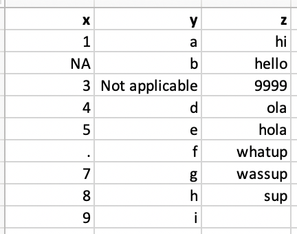
read_csv("data/df-na.csv")

## # A tibble: 9 × 3
##   x     y              z     
##   <chr> <chr>          <chr> 
## 1 1     a              hi    
## 2 <NA>  b              hello 
## 3 3     Not applicable 9999  
## 4 4     d              ola   
## 5 5     e              hola  
## 6 .     f              whatup
## 7 7     g              wassup
## 8 8     h              sup   
## 9 9     i              <NA>

13 / 32

Option 1. Explicit NAs

read_csv("data/df-na.csv", 
         na = c("", "NA", ".", "9999", "Not applicable"))

## # A tibble: 9 × 3
##       x y     z     
##   <dbl> <chr> <chr> 
## 1     1 a     hi    
## 2    NA b     hello 
## 3     3 <NA>  <NA>  
## 4     4 d     ola   
## 5     5 e     hola  
## 6    NA f     whatup
## 7     7 g     wassup
## 8     8 h     sup   
## 9     9 i     <NA>

14 / 32

Option 2. Specify column types

read_csv("data/df-na.csv", col_types = list(col_double(), 
                                            col_character(), 
                                            col_character()))

## Warning: One or more parsing issues, see `problems()` for details

## # A tibble: 9 × 3
##       x y              z     
##   <dbl> <chr>          <chr> 
## 1     1 a              hi    
## 2    NA b              hello 
## 3     3 Not applicable 9999  
## 4     4 d              ola   
## 5     5 e              hola  
## 6    NA f              whatup
## 7     7 g              wassup
## 8     8 h              sup   
## 9     9 i              <NA>

15 / 32

Column types

type function	data type
`col_character()`	character
`col_date()`	date
`col_datetime()`	POSIXct (date-time)
`col_double()`	double (numeric)
`col_factor()`	factor
`col_guess()`	let readr guess (default)
`col_integer()`	integer
`col_logical()`	logical
`col_number()`	numbers mixed with non-number characters
`col_numeric()`	double or integer
`col_skip()`	do not read
`col_time()`	time

16 / 32

Wondering where you remember these from?

read_csv("data/df-na.csv")

## Rows: 9 Columns: 3
## ── Column specification ─────────────────────────────────────────
## Delimiter: ","
## chr (3): x, y, z
## 
## ℹ Use `spec()` to retrieve the full column specification for this data.
## ℹ Specify the column types or set `show_col_types = FALSE` to quiet this message.

## # A tibble: 9 × 3
##   x     y              z     
##   <chr> <chr>          <chr> 
## 1 1     a              hi    
## 2 <NA>  b              hello 
## 3 3     Not applicable 9999  
## 4 4     d              ola   
...

17 / 32

Case study: Favourite foods

18 / 32

Favourite foods

19 / 32

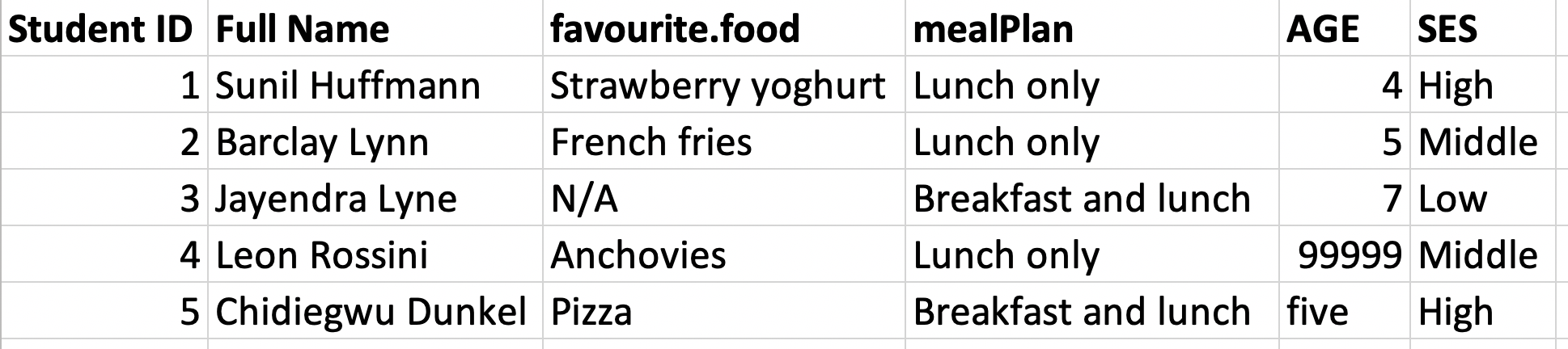
Favourite foods

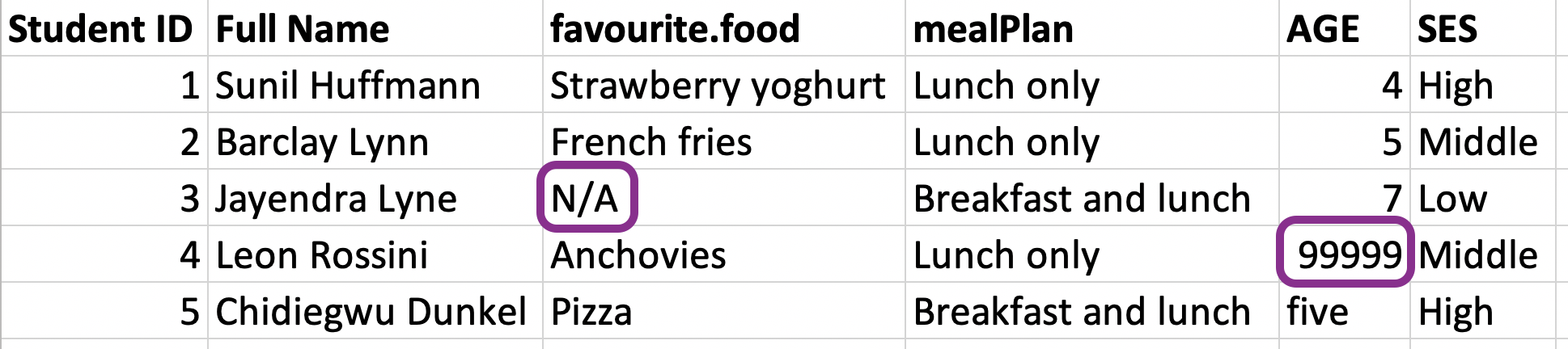
fav_food <- read_excel("data/favourite-food.xlsx")
fav_food

## # A tibble: 5 × 6
##   `Student ID` `Full Name`    favourite.food mealPlan AGE   SES  
##          <dbl> <chr>          <chr>          <chr>    <chr> <chr>
## 1            1 Sunil Huffmann Strawberry yo… Lunch o… 4     High 
## 2            2 Barclay Lynn   French fries   Lunch o… 5     Midd…
## 3            3 Jayendra Lyne  N/A            Breakfa… 7     Low  
## 4            4 Leon Rossini   Anchovies      Lunch o… 99999 Midd…
## 5            5 Chidiegwu Dun… Pizza          Breakfa… five  High

19 / 32

Variable names

20 / 32

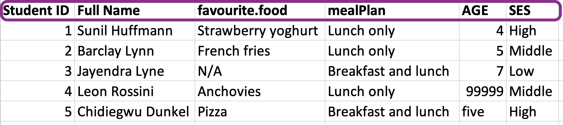
Variable names

fav_food <- read_excel("data/favourite-food.xlsx") %>%
  janitor::clean_names()
fav_food

## # A tibble: 5 × 6
##   student_id full_name       favourite_food meal_plan age   ses  
##        <dbl> <chr>           <chr>          <chr>     <chr> <chr>
## 1          1 Sunil Huffmann  Strawberry yo… Lunch on… 4     High 
## 2          2 Barclay Lynn    French fries   Lunch on… 5     Midd…
## 3          3 Jayendra Lyne   N/A            Breakfas… 7     Low  
## 4          4 Leon Rossini    Anchovies      Lunch on… 99999 Midd…
## 5          5 Chidiegwu Dunk… Pizza          Breakfas… five  High

20 / 32

Handling NAs

21 / 32

Handling NAs

fav_food <- read_excel("data/favourite-food.xlsx",
                       na = c("N/A", "99999")) %>%
  janitor::clean_names()
fav_food

## # A tibble: 5 × 6
##   student_id full_name       favourite_food meal_plan age   ses  
##        <dbl> <chr>           <chr>          <chr>     <chr> <chr>
## 1          1 Sunil Huffmann  Strawberry yo… Lunch on… 4     High 
## 2          2 Barclay Lynn    French fries   Lunch on… 5     Midd…
## 3          3 Jayendra Lyne   <NA>           Breakfas… 7     Low  
## 4          4 Leon Rossini    Anchovies      Lunch on… <NA>  Midd…
## 5          5 Chidiegwu Dunk… Pizza          Breakfas… five  High

21 / 32

Make `age` numeric

fav_food <- fav_food %>%
  mutate(
    age = if_else(age == "five", "5", age),
    age = as.numeric(age)
    )
glimpse(fav_food)

## Rows: 5
## Columns: 6
## $ student_id     <dbl> 1, 2, 3, 4, 5
## $ full_name      <chr> "Sunil Huffmann", "Barclay Lynn", "Jayen…
## $ favourite_food <chr> "Strawberry yoghurt", "French fries", NA…
## $ meal_plan      <chr> "Lunch only", "Lunch only", "Breakfast a…
## $ age            <dbl> 4, 5, 7, NA, 5
## $ ses            <chr> "High", "Middle", "Low", "Middle", "High"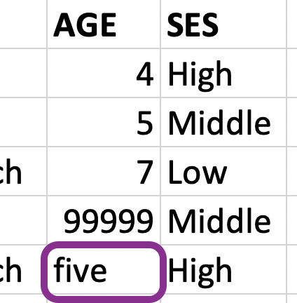

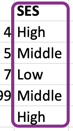
22 / 32

Socio-economic status

What order are the levels of ses listed in?

fav_food %>%
  count(ses)

## # A tibble: 3 × 2
##   ses        n
##   <chr>  <int>
## 1 High       2
## 2 Low        1
## 3 Middle     2

23 / 32

datasciencebox.org

Make ses factorfav_food <- fav_food %>%
  mutate(ses = fct_relevel(ses, "Low", "Middle", "High"))
fav_food %>%
  count(ses)

## # A tibble: 3 × 2
##   ses        n
##   <fct>  <int>
## 1 Low        1
## 2 Middle     2
## 3 High       2
24 / 32

Putting it altogether

fav_food <- read_excel("data/favourite-food.xlsx", na = c("N/A", "99999")) %>%
  janitor::clean_names() %>%
  mutate(
    age = if_else(age == "five", "5", age), 
    age = as.numeric(age),
    ses = fct_relevel(ses, "Low", "Middle", "High")
  )
fav_food

## # A tibble: 5 × 6
##   student_id full_name       favourite_food meal_plan   age ses  
##        <dbl> <chr>           <chr>          <chr>     <dbl> <fct>
## 1          1 Sunil Huffmann  Strawberry yo… Lunch on…     4 High 
## 2          2 Barclay Lynn    French fries   Lunch on…     5 Midd…
## 3          3 Jayendra Lyne   <NA>           Breakfas…     7 Low  
## 4          4 Leon Rossini    Anchovies      Lunch on…    NA Midd…
## 5          5 Chidiegwu Dunk… Pizza          Breakfas…     5 High

25 / 32

Out and back in

write_csv(fav_food, file = "data/fav-food-clean.csv")
fav_food_clean <- read_csv("data/fav-food-clean.csv")

26 / 32

What happened to ses again?

fav_food_clean %>%
  count(ses)

## # A tibble: 3 × 2
##   ses        n
##   <chr>  <int>
## 1 High       2
## 2 Low        1
## 3 Middle     2

27 / 32

`read_rds()` and `write_rds()`

CSVs can be unreliable for saving interim results if there is specific variable type information you want to hold on to.
An alternative is RDS files, you can read and write them with read_rds() and write_rds(), respectively.

read_rds(path)
write_rds(x, path)

28 / 32

Out and back in, take 2

write_rds(fav_food, file = "data/fav-food-clean.rds")
fav_food_clean <- read_rds("data/fav-food-clean.rds")
fav_food_clean %>%
  count(ses)

## # A tibble: 3 × 2
##   ses        n
##   <fct>  <int>
## 1 Low        1
## 2 Middle     2
## 3 High       2

29 / 32

Other types of data

30 / 32

Other types of data

googlesheets4: Google Sheets
haven: SPSS, Stata, and SAS files
DBI, along with a database specific backend (e.g. RMySQL, RSQLite, RPostgreSQL etc): allows you to run SQL queries against a database and return a data frame
jsonline: JSON
xml2: xml
rvest: web scraping
httr: web APIs
sparklyr: data loaded into spark

31 / 32

Your turn!

RStudio Cloud > AE 06 - Nobels and sales + Data import > sales-excel.Rmd.
Load the sales.xlsx file from the data-raw/ folder, using appropriate arguments for the read_excel() function such that it looks like the output on the left.
Stretch goal: Manipulate the sales data such that it looks like the output on the right.

## # A tibble: 9 × 2
##   id      n    
##   <chr>   <chr>
## 1 Brand 1 n    
## 2 1234    8    
## 3 8721    2    
## 4 1822    3    
## 5 Brand 2 n    
## 6 3333    1    
## # … with 3 more rows

## # A tibble: 7 × 3
##   brand      id     n
##   <chr>   <dbl> <dbl>
## 1 Brand 1  1234     8
## 2 Brand 1  8721     2
## 3 Brand 1  1822     3
## 4 Brand 2  3333     1
## 5 Brand 2  2156     3
## 6 Brand 2  3987     6
## # … with 1 more row

↑, ←, Pg Up, k	Go to previous slide
↓, →, Pg Dn, Space, j	Go to next slide
Home	Go to first slide
End	Go to last slide
Number + Return	Go to specific slide
b / m / f	Toggle blackout / mirrored / fullscreen mode
c	Clone slideshow
p	Toggle presenter mode
t	Restart the presentation timer
?, h	Toggle this help

Importing data

Data Science in a Box

datasciencebox.org

Reading rectangular data into R

readr

readr

readxl

Reading data

Writing data

Writing data

Your turn!

Variable names

Data with bad names

Data with bad names

Option 1 - Define column names

Option 2 - Format text to snake_case

Variable types

Option 1. Explicit NAs

Option 2. Specify column types

Column types

Case study: Favourite foods

Favourite foods

Favourite foods

Variable names

Variable names

Handling NAs

Handling NAs

Make `age` numeric

Socio-economic status

Make `ses` factor

Putting it altogether

Out and back in

`read_rds()` and `write_rds()`

Out and back in, take 2

Other types of data

Other types of data

Your turn!

Reading rectangular data into R

Help

Importing data

Data Science in a Box

datasciencebox.org

Reading rectangular data into R

readr

readr

readxl

Reading data

Writing data

Writing data

Your turn!

Variable names

Data with bad names

Data with bad names

Option 1 - Define column names

Option 2 - Format text to snake_case

Variable types

Option 1. Explicit NAs

Option 2. Specify column types

Column types

Case study: Favourite foods

Favourite foods

Favourite foods

Variable names

Variable names

Handling NAs

Handling NAs

Make age numeric

Socio-economic status

Make ses factor

Putting it altogether

Out and back in

read_rds() and write_rds()

Out and back in, take 2

Other types of data

Other types of data

Your turn!

Reading rectangular data into R

Help

Make `age` numeric

Make `ses` factor

`read_rds()` and `write_rds()`