Data: Paris Paintings

pp <- read_csv("data/paris-paintings.csv", na = c("n/a", "", "NA"))

• Number of observations: 3393
• Number of variables: 61

Goal: Predict height from width

$${\widehat{height}}_i={\beta }_0+{\beta }_1\times widt{h}_i$$

Step 1: Specify model

linear_reg()

## Linear Regression Model Specification (regression)
## 
## Computational engine: lm

Step 2: Set model fitting engine

linear_reg() %>%
  set_engine("lm") # lm: linear model

## Linear Regression Model Specification (regression)
## 
## Computational engine: lm

Step 3: Fit model & estimate parameters

... using formula syntax

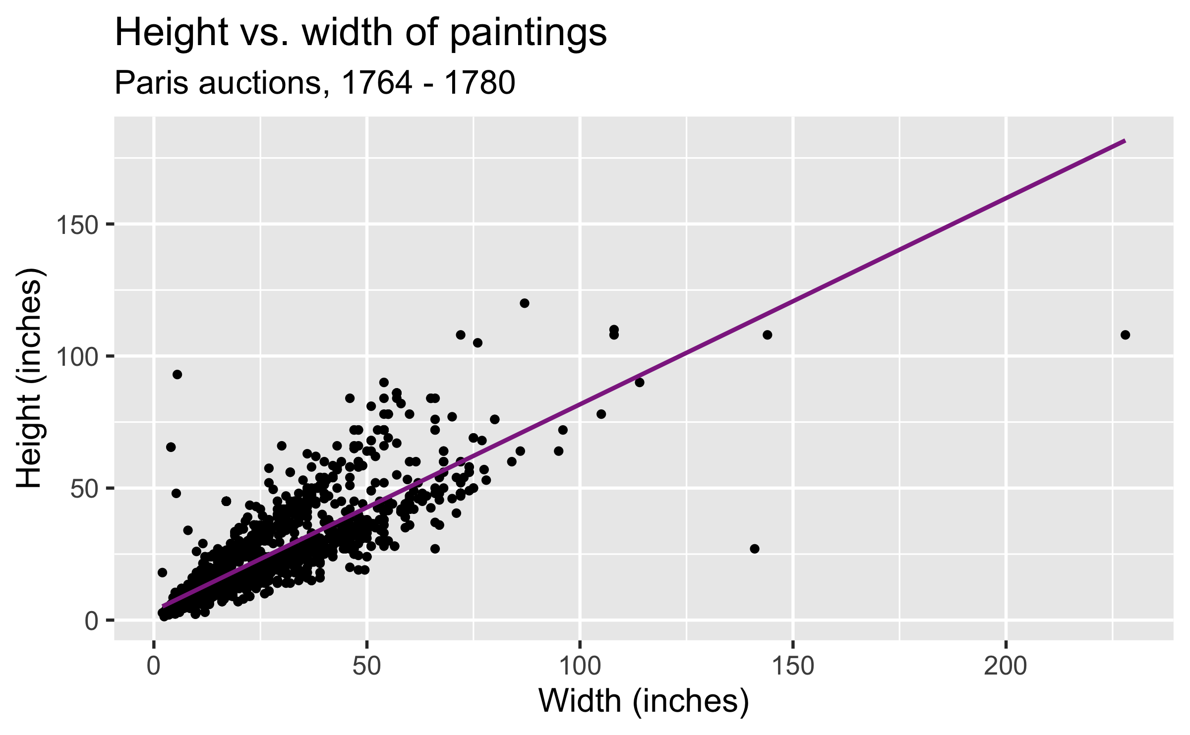
linear_reg() %>%
  set_engine("lm") %>%
  fit(Height_in ~ Width_in, data = pp)

## parsnip model object
## 
## 
## Call:
## stats::lm(formula = Height_in ~ Width_in, data = data)
## 
## Coefficients:
## (Intercept)     Width_in  
##      3.6214       0.7808

A closer look at model output

## parsnip model object
## 
## 
## Call:
## stats::lm(formula = Height_in ~ Width_in, data = data)
## 
## Coefficients:
## (Intercept)     Width_in  
##      3.6214       0.7808

A tidy look at model output

linear_reg() %>%
  set_engine("lm") %>%
  fit(Height_in ~ Width_in, data = pp) %>%
  tidy()

## # A tibble: 2 × 5
##   term        estimate std.error statistic  p.value
##   <chr>          <dbl>     <dbl>     <dbl>    <dbl>
## 1 (Intercept)    3.62    0.254        14.3 8.82e-45
## 2 Width_in       0.781   0.00950      82.1 0

Slope and intercept

• Slope: For each additional inch the painting is wider, the height is expected to be higher, on average, by 0.781 inches.
• Intercept: Paintings that are 0 inches wide are expected to be 3.62 inches high, on average. (Does this make sense?)

Correlation does not imply causation

Remember this when interpreting model coefficients

Linear model with a single predictor

• We're interested in ${\beta }_0$ (population parameter for the intercept) and ${\beta }_1$ (population parameter for the slope) in the following model:

$${\hat{y}}_i={\beta }_0+{\beta }_1{x}_i$$

• Tough luck, you can't have them...
• So we use sample statistics to estimate them:

$${\hat{y}}_i=b_0+b_1{x}_i$$

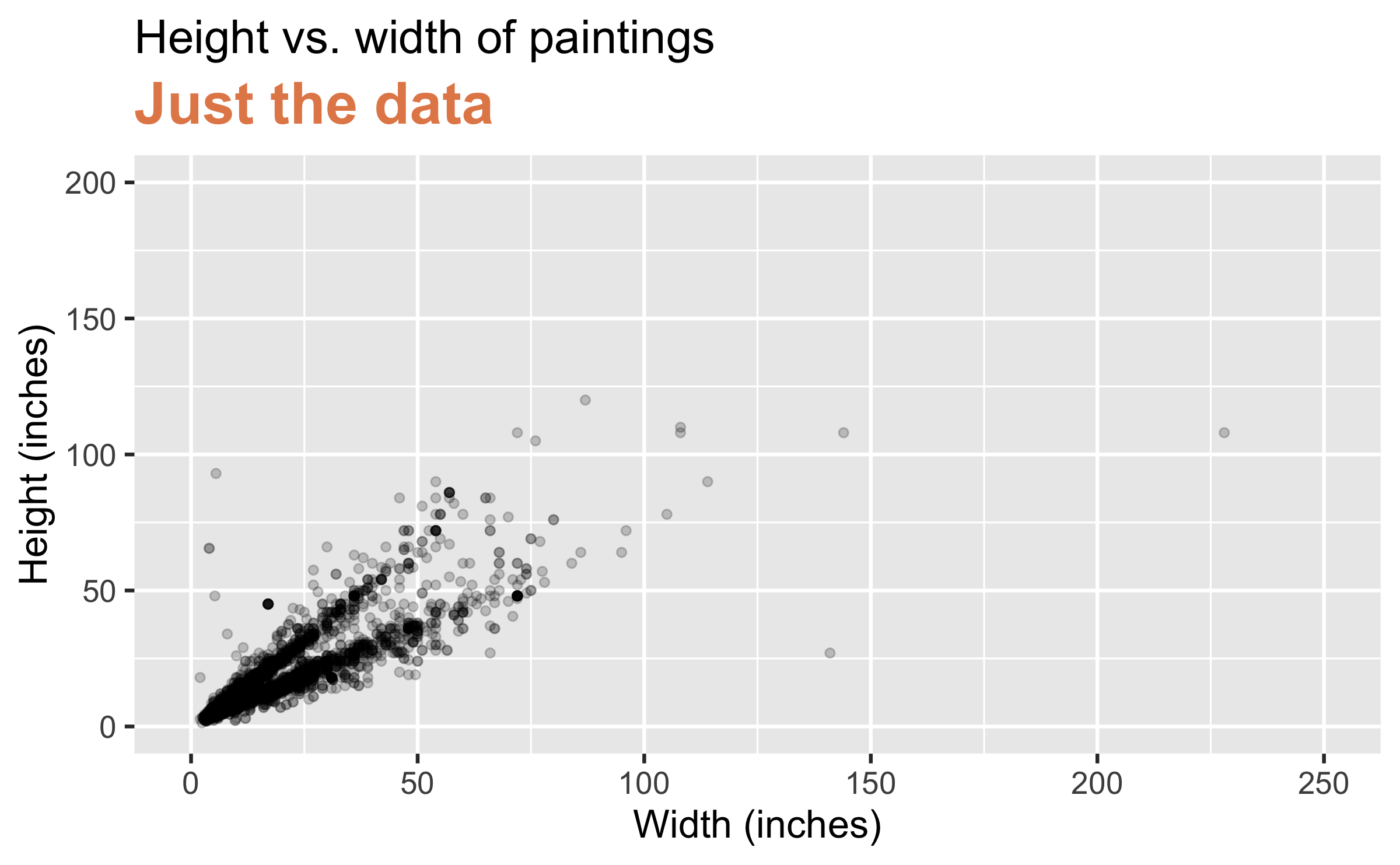
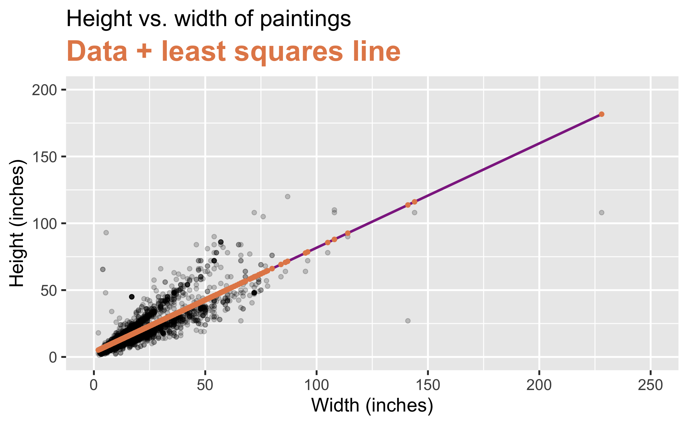
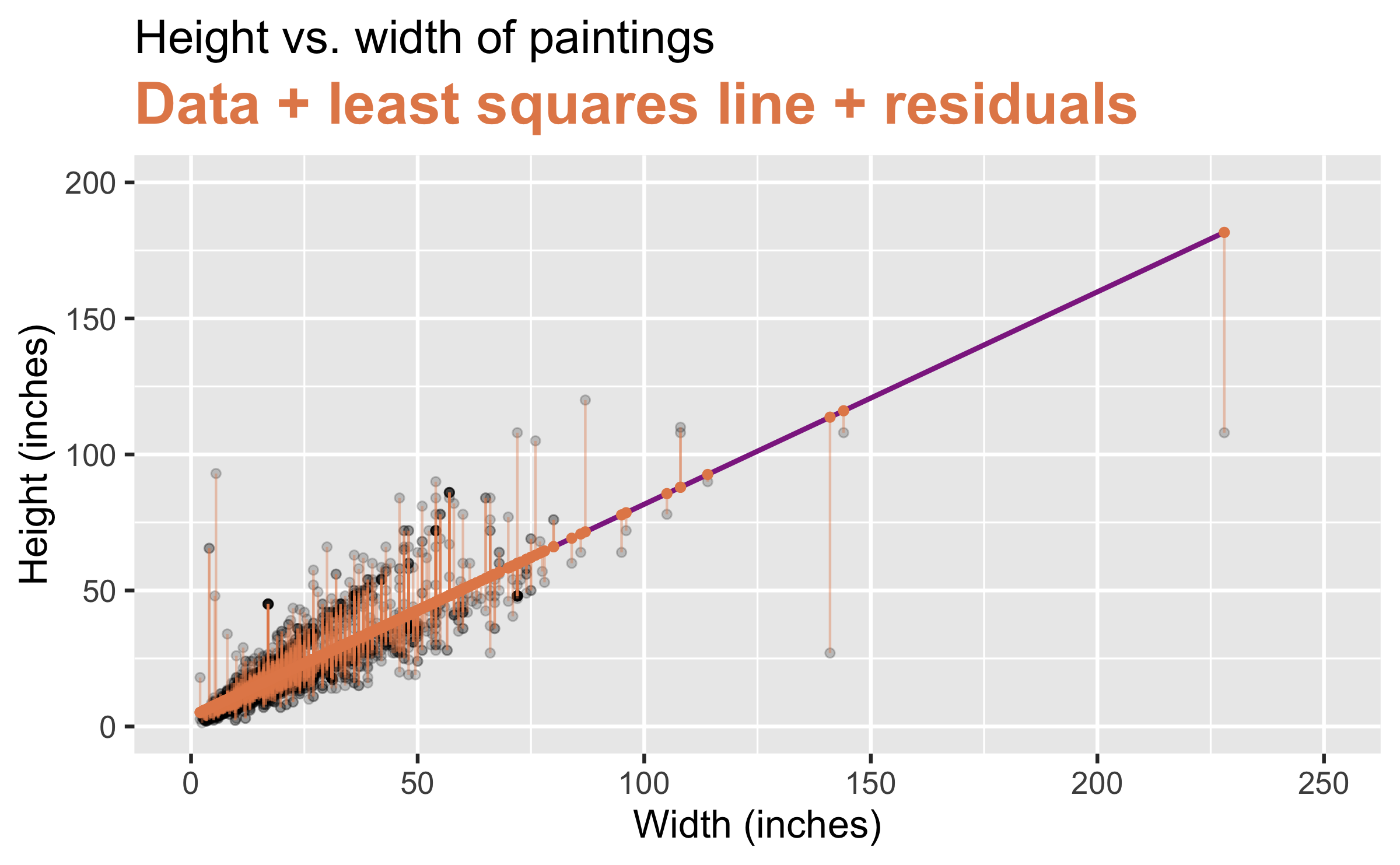
Least squares regression

• The regression line minimizes the sum of squared residuals.
• If $e_i=y_i-{\hat{y}}_i$, then, the regression line minimizes ${\sum }_{i=1}^n{e}_i^2$.

Visualizing residuals

Visualizing residuals (cont.)

Visualizing residuals (cont.)

Properties of least squares regression

• The regression line goes through the center of mass point, the coordinates corresponding to average $x$ and average $y$, $(\overline{x},\overline{y})$:

$$\overline{y}=b_0+b_1\overline{x}\to b_0=\overline{y}-b_1\overline{x}$$

• The slope has the same sign as the correlation coefficient: $b_1=r\frac{s_y}{s_x}$
• The sum of the residuals is zero: ${\sum }_{i=1}^n{e}_i=0$
• The residuals and $x$ values are uncorrelated

Categorical predictor with 2 levels

## # A tibble: 3,393 × 3
##    name      Height_in landsALL
##    <chr>         <dbl>    <dbl>
##  1 L1764-2          37        0
##  2 L1764-3          18        0
##  3 L1764-4          13        1
##  4 L1764-5a         14        1
##  5 L1764-5b         14        1
##  6 L1764-6           7        0
##  7 L1764-7a          6        0
##  8 L1764-7b          6        0
##  9 L1764-8          15        0
## 10 L1764-9a          9        0
## 11 L1764-9b          9        0
## 12 L1764-10a        16        1
## 13 L1764-10b        16        1
## 14 L1764-10c        16        1
## 15 L1764-11         20        0
## 16 L1764-12a        14        1
## 17 L1764-12b        14        1
## 18 L1764-13a        15        1
## 19 L1764-13b        15        1
## 20 L1764-14         37        0
## # … with 3,373 more rows

Height & landscape features

linear_reg() %>%
  set_engine("lm") %>%
  fit(Height_in ~ factor(landsALL), data = pp) %>%
  tidy()

## # A tibble: 2 × 5
##   term              estimate std.error statistic  p.value
##   <chr>                <dbl>     <dbl>     <dbl>    <dbl>
## 1 (Intercept)          22.7      0.328      69.1 0       
## 2 factor(landsALL)1    -5.65     0.532     -10.6 7.97e-26

Height & landscape features

$$\widehat{Heigh{t}_{in}}=22.7-5.645landsALL$$

• Slope: Paintings with landscape features are expected, on average, to be 5.645 inches shorter than paintings that without landscape features

  • Compares baseline level (landsALL = 0) to the other level (landsALL = 1)

• Intercept: Paintings that don't have landscape features are expected, on average, to be 22.7 inches tall

Relationship between height and school

linear_reg() %>%
  set_engine("lm") %>%
  fit(Height_in ~ school_pntg, data = pp) %>%
  tidy()

## # A tibble: 7 × 5
##   term            estimate std.error statistic p.value
##   <chr>              <dbl>     <dbl>     <dbl>   <dbl>
## 1 (Intercept)        14.0       10.0     1.40  0.162  
## 2 school_pntgD/FL     2.33      10.0     0.232 0.816  
## 3 school_pntgF       10.2       10.0     1.02  0.309  
## 4 school_pntgG        1.65      11.9     0.139 0.889  
## 5 school_pntgI       10.3       10.0     1.02  0.306  
## 6 school_pntgS       30.4       11.4     2.68  0.00744
## 7 school_pntgX        2.87      10.3     0.279 0.780

Dummy variables

## # A tibble: 7 × 5
##   term            estimate std.error statistic p.value
##   <chr>              <dbl>     <dbl>     <dbl>   <dbl>
## 1 (Intercept)        14.0       10.0     1.40  0.162  
## 2 school_pntgD/FL     2.33      10.0     0.232 0.816  
## 3 school_pntgF       10.2       10.0     1.02  0.309  
## 4 school_pntgG        1.65      11.9     0.139 0.889  
## 5 school_pntgI       10.3       10.0     1.02  0.306  
## 6 school_pntgS       30.4       11.4     2.68  0.00744
## 7 school_pntgX        2.87      10.3     0.279 0.780

• When the categorical explanatory variable has many levels, they're encoded to dummy variables
• Each coefficient describes the expected difference between heights in that particular school compared to the baseline level

Categorical predictor with 3+ levels

## # A tibble: 3,393 × 3
##    name      Height_in school_pntg
##    <chr>         <dbl> <chr>      
##  1 L1764-2          37 F          
##  2 L1764-3          18 I          
##  3 L1764-4          13 D/FL       
##  4 L1764-5a         14 F          
##  5 L1764-5b         14 F          
##  6 L1764-6           7 I          
##  7 L1764-7a          6 F          
##  8 L1764-7b          6 F          
##  9 L1764-8          15 I          
## 10 L1764-9a          9 D/FL       
## 11 L1764-9b          9 D/FL       
## 12 L1764-10a        16 X          
## 13 L1764-10b        16 X          
## 14 L1764-10c        16 X          
## 15 L1764-11         20 D/FL       
## 16 L1764-12a        14 D/FL       
## 17 L1764-12b        14 D/FL       
## 18 L1764-13a        15 D/FL       
## 19 L1764-13b        15 D/FL       
## 20 L1764-14         37 F          
## # … with 3,373 more rows

Relationship between height and school

## # A tibble: 7 × 5
##   term            estimate std.error statistic p.value
##   <chr>              <dbl>     <dbl>     <dbl>   <dbl>
## 1 (Intercept)        14.0       10.0     1.40  0.162  
## 2 school_pntgD/FL     2.33      10.0     0.232 0.816  
## 3 school_pntgF       10.2       10.0     1.02  0.309  
## 4 school_pntgG        1.65      11.9     0.139 0.889  
## 5 school_pntgI       10.3       10.0     1.02  0.306  
## 6 school_pntgS       30.4       11.4     2.68  0.00744
## 7 school_pntgX        2.87      10.3     0.279 0.780