The data

pp <- read_csv(
  "data/paris-paintings.csv",
  na = c("n/a", "", "NA")
) %>%
  mutate(log_price = log(price))

Multiple predictors

• Response variable: log_price
• Explanatory variables: Width and height

pp_fit <- linear_reg() %>%
  set_engine("lm") %>%
  fit(log_price ~ Width_in + Height_in, data = pp)
tidy(pp_fit)

## # A tibble: 3 × 5
##   term        estimate std.error statistic  p.value
##   <chr>          <dbl>     <dbl>     <dbl>    <dbl>
## 1 (Intercept)   4.77     0.0579      82.4  0       
## 2 Width_in      0.0269   0.00373      7.22 6.58e-13
## 3 Height_in    -0.0133   0.00395     -3.36 7.93e- 4

Linear model with multiple predictors

## # A tibble: 3 × 5
##   term        estimate std.error statistic  p.value
##   <chr>          <dbl>     <dbl>     <dbl>    <dbl>
## 1 (Intercept)   4.77     0.0579      82.4  0       
## 2 Width_in      0.0269   0.00373      7.22 6.58e-13
## 3 Height_in    -0.0133   0.00395     -3.36 7.93e- 4

$$\widehat{log\_price}=4.77+0.0269\times width-0.0133\times height$$

Visualizing models with multiple predictors

p <- plot_ly(pp,
  x = ~Width_in, y = ~Height_in, z = ~log_price,
  marker = list(size = 3, color = "lightgray", alpha = 0.5, 
                line = list(color = "gray", width = 2))) %>%
  add_markers() %>%
  plotly::layout(scene = list(
    xaxis = list(title = "Width (in)"),
    yaxis = list(title = "Height (in)"),
    zaxis = list(title = "log_price")
  )) %>%
  config(displayModeBar = FALSE)
frameWidget(p)

Price, surface area, and living artist

• Explore the relationship between price of paintings and surface area, conditioned on whether or not the artist is still living
• First visualize and explore, then model
• But first, prep the data

pp <- pp %>%
  mutate(artistliving = if_else(artistliving == 0, "Deceased", "Living"))
pp %>%
  count(artistliving)

## # A tibble: 2 × 2
##   artistliving     n
##   <chr>        <int>
## 1 Deceased      2937
## 2 Living         456

Typical surface area

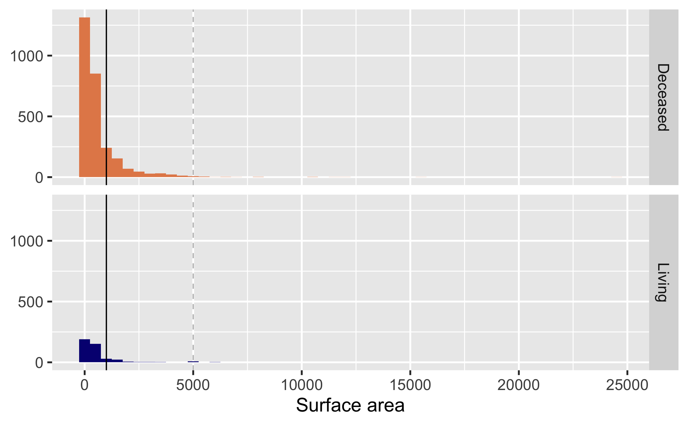
ggplot(data = pp, aes(x = Surface, fill = artistliving)) +
  geom_histogram(binwidth = 500) + 
  facet_grid(artistliving ~ .) +
  scale_fill_manual(values = c("#E48957", "#071381")) +
  guides(fill = "none") +
  labs(x = "Surface area", y = NULL) +
  geom_vline(xintercept = 1000) +
  geom_vline(xintercept = 5000, linetype = "dashed", color = "gray")

## Warning: Removed 176 rows containing non-finite values
## (stat_bin).

Narrowing the scope

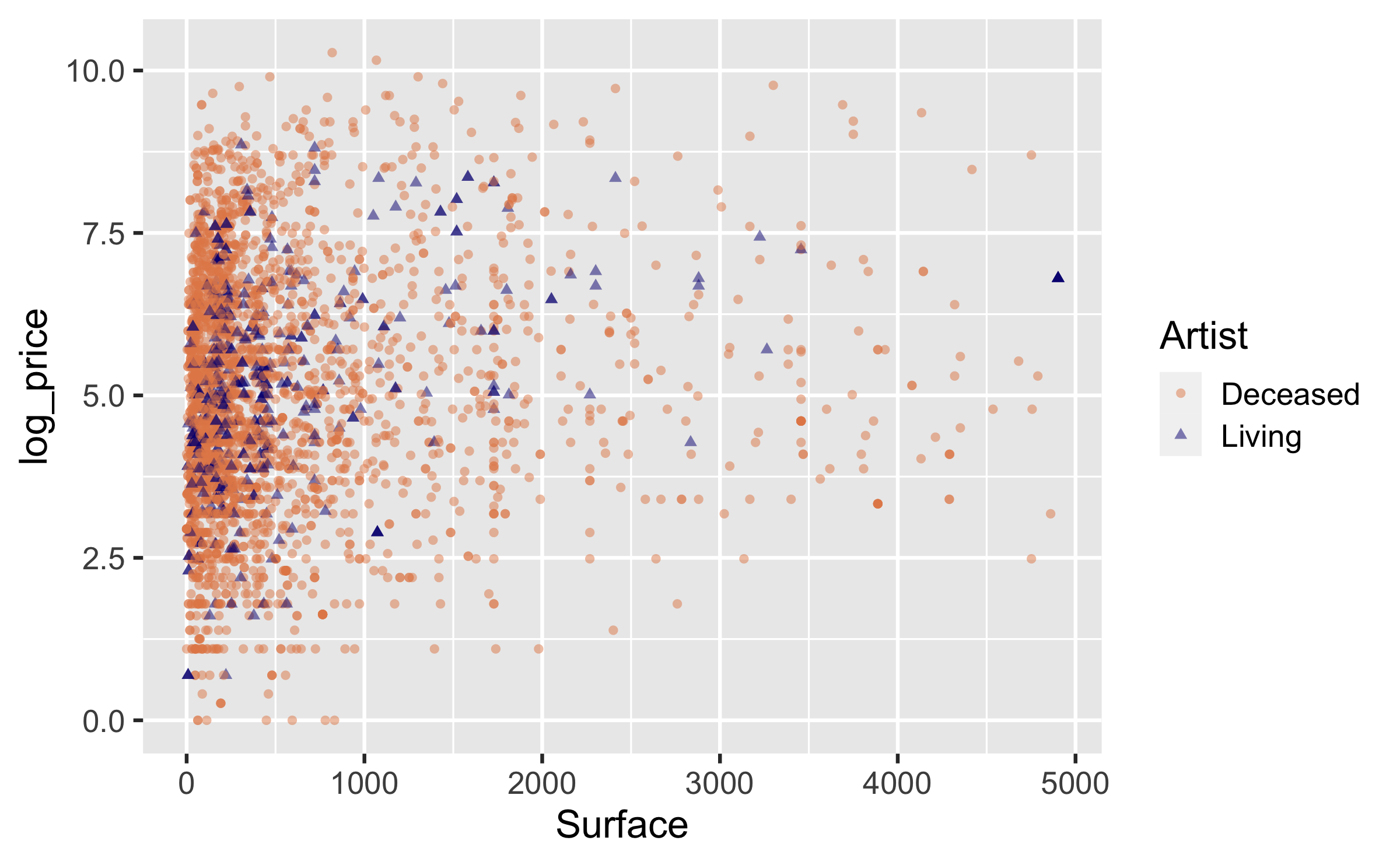
pp_Surf_lt_5000 <- pp %>%
  filter(Surface < 5000)
ggplot(data = pp_Surf_lt_5000, 
       aes(y = log_price, x = Surface, color = artistliving, shape = artistliving)) +
  geom_point(alpha = 0.5) +
  labs(color = "Artist", shape = "Artist") +
  scale_color_manual(values = c("#E48957", "#071381"))

Facet to get a better look

ggplot(data = pp_Surf_lt_5000, 
       aes(y = log_price, x = Surface, color = artistliving, shape = artistliving)) +
  geom_point(alpha = 0.5) +
  facet_wrap(~artistliving) +
  scale_color_manual(values = c("#E48957", "#071381")) +
  labs(color = "Artist", shape = "Artist")

Two ways to model

• Main effects: Assuming relationship between surface and logged price does not vary by whether or not the artist is living.
• Interaction effects: Assuming relationship between surface and logged price varies by whether or not the artist is living.

Interacting explanatory variables

• Including an interaction effect in the model allows for different slopes, i.e. nonparallel lines.
• This implies that the regression coefficient for an explanatory variable would change as another explanatory variable changes.
• This can be accomplished by adding an interaction variable: the product of two explanatory variables.

Two ways to model

Fit model with main effects

• Response variable: log_price
• Explanatory variables: Surface area and artistliving

pp_main_fit <- linear_reg() %>%
  set_engine("lm") %>%
  fit(log_price ~ Surface + artistliving, data = pp_Surf_lt_5000)
tidy(pp_main_fit)

## # A tibble: 3 × 5
##   term               estimate std.error statistic  p.value
##   <chr>                 <dbl>     <dbl>     <dbl>    <dbl>
## 1 (Intercept)        4.88     0.0424       115.   0       
## 2 Surface            0.000265 0.0000415      6.39 1.85e-10
## 3 artistlivingLiving 0.137    0.0970         1.41 1.57e- 1

$$\widehat{log\_price}=4.88+0.000265\times surface+0.137\times artistliving$$

Solving the model

• Non-living artist: Plug in 0 for artistliving

$\widehat{log\_price}=4.88+0.000265\times surface+0.137\times 0$
$=4.88+0.000265\times surface$

• Living artist: Plug in 1 for artistliving

$\widehat{log\_price}=4.88+0.000265\times surface+0.137\times 1$
$=5.017+0.000265\times surface$

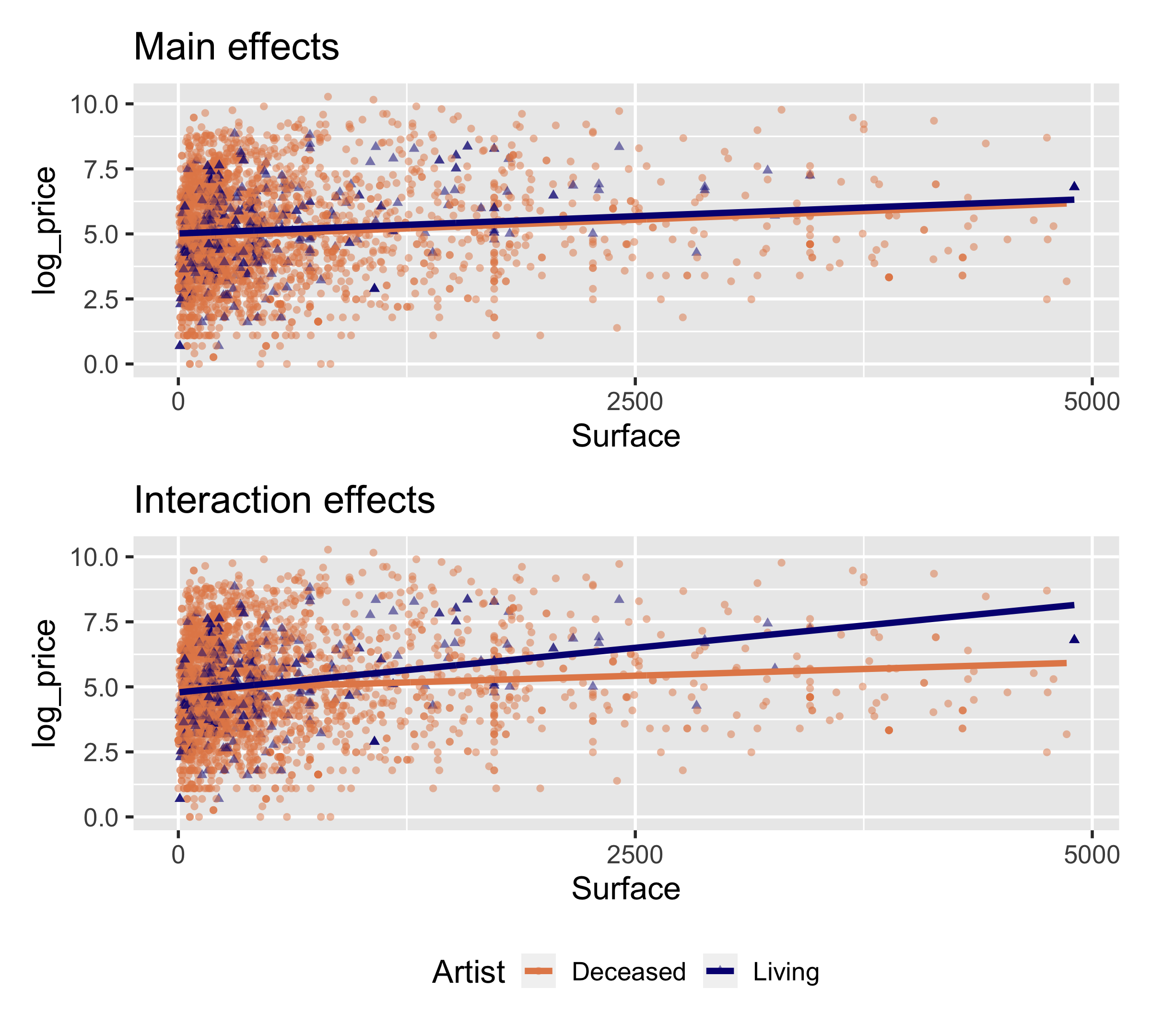
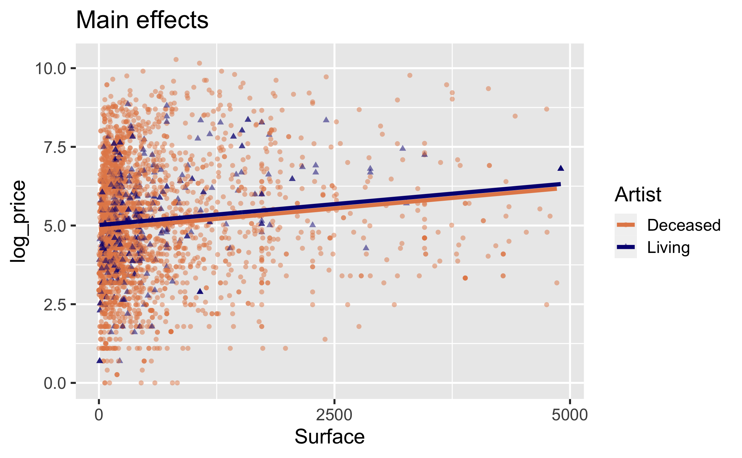
Visualizing main effects

Interpreting main effects

tidy(pp_main_fit) %>% 
  mutate(exp_estimate = exp(estimate)) %>%
  select(term, estimate, exp_estimate)

## # A tibble: 3 × 3
##   term               estimate exp_estimate
##   <chr>                 <dbl>        <dbl>
## 1 (Intercept)        4.88           132.  
## 2 Surface            0.000265         1.00
## 3 artistlivingLiving 0.137            1.15

• All else held constant, for each additional square inch in painting's surface area, the price of the painting is predicted, on average, to be higher by a factor of 1.
• All else held constant, paintings by a living artist are predicted, on average, to be higher by a factor of 1.15 compared to paintings by an artist who is no longer alive.
• Paintings that are by an artist who is not alive and that have a surface area of 0 square inches are predicted, on average, to be 132 livres.

Main vs. interaction effects

• The way we specified our main effects model only lets artistliving affect the intercept.
• Model implicitly assumes that paintings with living and deceased artists have the same slope and only allows for different intercepts.

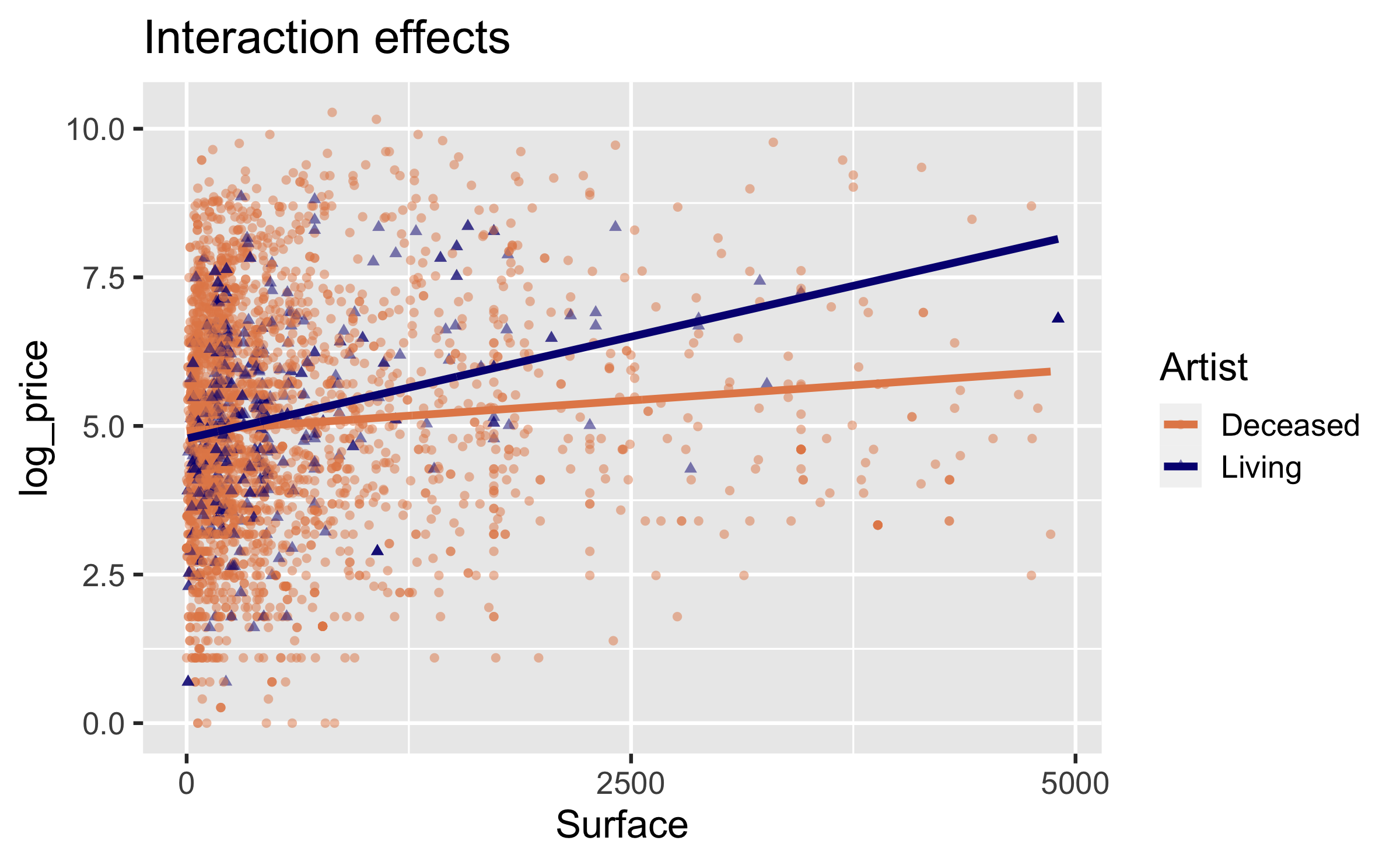
Interaction: Surface * artistliving

Fit model with interaction effects

• Response variable: log_price
• Explanatory variables: Surface area, artistliving, and their interaction

pp_int_fit <- linear_reg() %>%
  set_engine("lm") %>%
  fit(log_price ~ Surface * artistliving, data = pp_Surf_lt_5000)
tidy(pp_int_fit)

## # A tibble: 4 × 5
##   term                       estimate std.error statistic p.value
##   <chr>                         <dbl>     <dbl>     <dbl>   <dbl>
## 1 (Intercept)                 4.91e+0 0.0432       114.   0      
## 2 Surface                     2.06e-4 0.0000442      4.65 3.37e-6
## 3 artistlivingLiving         -1.26e-1 0.119         -1.06 2.89e-1
## 4 Surface:artistlivingLiving  4.79e-4 0.000126       3.81 1.39e-4

Linear model with interaction effects

## # A tibble: 4 × 5
##   term                       estimate std.error statistic p.value
##   <chr>                         <dbl>     <dbl>     <dbl>   <dbl>
## 1 (Intercept)                 4.91e+0 0.0432       114.   0      
## 2 Surface                     2.06e-4 0.0000442      4.65 3.37e-6
## 3 artistlivingLiving         -1.26e-1 0.119         -1.06 2.89e-1
## 4 Surface:artistlivingLiving  4.79e-4 0.000126       3.81 1.39e-4

$$\widehat{log\_price}=4.91+0.00021\times surface-0.126\times artistliving$$ $$+0.00048\times surface\ast artistliving$$

Interpretation of interaction effects

• Rate of change in price as the surface area of the painting increases does vary between paintings by living and non-living artists (different slopes),
• Some paintings by living artists are more expensive than paintings by non-living artists, and some are not (different intercept).

Comparing models

It appears that adding the interaction actually increased adjusted $R^2$, so we should indeed use the model with the interactions.

glance(pp_main_fit)$adj.r.squared

## [1] 0.01258977

glance(pp_int_fit)$adj.r.squared

## [1] 0.01676753

Third order interactions

• Can you? Yes
• Should you? Probably not if you want to interpret these interactions in context of the data.