Feature engineering
- We prefer simple models when possible, but parsimony does not mean sacrificing accuracy (or predictive performance) in the interest of simplicity
3 / 26
Feature engineering
- We prefer simple models when possible, but parsimony does not mean sacrificing accuracy (or predictive performance) in the interest of simplicity
- Variables that go into the model and how they are represented are just as critical to success of the model
3 / 26
Feature engineering
- We prefer simple models when possible, but parsimony does not mean sacrificing accuracy (or predictive performance) in the interest of simplicity
- Variables that go into the model and how they are represented are just as critical to success of the model
- Feature engineering allows us to get creative with our predictors in an effort to make them more useful for our model (to increase its predictive performance)
3 / 26
Same training and testing sets as before
# Fix random numbers by setting the seed # Enables analysis to be reproducible when random numbers are used set.seed(1116)# Put 80% of the data into the training set email_split <- initial_split(email, prop = 0.80)# Create data frames for the two sets:train_data <- training(email_split)test_data <- testing(email_split)4 / 26
A simple approach: mutate()
train_data %>% mutate( date = lubridate::date(time), dow = wday(time), month = month(time) ) %>% select(time, date, dow, month) %>% sample_n(size = 5) # shuffle to show a variety## # A tibble: 5 × 4## time date dow month## <dttm> <date> <dbl> <dbl>## 1 2012-03-15 14:51:35 2012-03-15 5 3## 2 2012-03-03 09:24:02 2012-03-03 7 3## 3 2012-01-18 11:55:23 2012-01-18 4 1## 4 2012-02-24 23:08:59 2012-02-24 6 2## 5 2012-01-11 08:18:51 2012-01-11 4 15 / 26
Modeling workflow, revisited
- Create a recipe for feature engineering steps to be applied to the training data
6 / 26
Modeling workflow, revisited
- Create a recipe for feature engineering steps to be applied to the training data
- Fit the model to the training data after these steps have been applied
6 / 26
Modeling workflow, revisited
- Create a recipe for feature engineering steps to be applied to the training data
- Fit the model to the training data after these steps have been applied
- Using the model estimates from the training data, predict outcomes for the test data
6 / 26
Modeling workflow, revisited
- Create a recipe for feature engineering steps to be applied to the training data
- Fit the model to the training data after these steps have been applied
- Using the model estimates from the training data, predict outcomes for the test data
- Evaluate the performance of the model on the test data
6 / 26
Initiate a recipe
email_rec <- recipe( spam ~ ., # formula data = train_data # data to use for cataloguing names and types of variables )summary(email_rec)## # A tibble: 21 × 4## variable type role source ## <chr> <chr> <chr> <chr> ## 1 to_multiple nominal predictor original## 2 from nominal predictor original## 3 cc numeric predictor original## 4 sent_email nominal predictor original## 5 time date predictor original## 6 image numeric predictor original## 7 attach numeric predictor original## 8 dollar numeric predictor original## 9 winner nominal predictor original## 10 inherit numeric predictor original## 11 viagra numeric predictor original## 12 password numeric predictor original## 13 num_char numeric predictor original## 14 line_breaks numeric predictor original## 15 format nominal predictor original## 16 re_subj nominal predictor original## 17 exclaim_subj numeric predictor original## 18 urgent_subj nominal predictor original## 19 exclaim_mess numeric predictor original## 20 number nominal predictor original## 21 spam nominal outcome original8 / 26
Remove certain variables
email_rec <- email_rec %>% step_rm(from, sent_email)## Recipe## ## Inputs:## ## role #variables## outcome 1## predictor 20## ## Operations:## ## Variables removed from, sent_email9 / 26
Feature engineer date
email_rec <- email_rec %>% step_date(time, features = c("dow", "month")) %>% step_rm(time)## Recipe## ## Inputs:## ## role #variables## outcome 1## predictor 20## ## Operations:## ## Variables removed from, sent_email## Date features from time## Variables removed time10 / 26
Discretize numeric variables
email_rec <- email_rec %>% step_cut(cc, attach, dollar, breaks = c(0, 1)) %>% step_cut(inherit, password, breaks = c(0, 1, 5, 10, 20))## Recipe## ## Inputs:## ## role #variables## outcome 1## predictor 20## ## Operations:## ## Variables removed from, sent_email## Date features from time## Variables removed time## Cut numeric for cc, attach, dollar## Cut numeric for inherit, password11 / 26
Create dummy variables
email_rec <- email_rec %>% step_dummy(all_nominal(), -all_outcomes())## Recipe## ## Inputs:## ## role #variables## outcome 1## predictor 20## ## Operations:## ## Variables removed from, sent_email## Date features from time## Variables removed time## Cut numeric for cc, attach, dollar## Cut numeric for inherit, password## Dummy variables from all_nominal(), -all_outcomes()12 / 26
Remove zero variance variables
Variables that contain only a single value
email_rec <- email_rec %>% step_zv(all_predictors())## Recipe## ## Inputs:## ## role #variables## outcome 1## predictor 20## ## Operations:## ## Variables removed from, sent_email## Date features from time## Variables removed time## Cut numeric for cc, attach, dollar## Cut numeric for inherit, password## Dummy variables from all_nominal(), -all_outcomes()## Zero variance filter on all_predictors()13 / 26
All in one place
email_rec <- recipe(spam ~ ., data = email) %>% step_rm(from, sent_email) %>% step_date(time, features = c("dow", "month")) %>% step_rm(time) %>% step_cut(cc, attach, dollar, breaks = c(0, 1)) %>% step_cut(inherit, password, breaks = c(0, 1, 5, 10, 20)) %>% step_dummy(all_nominal(), -all_outcomes()) %>% step_zv(all_predictors())14 / 26
Define model
email_mod <- logistic_reg() %>% set_engine("glm")email_mod## Logistic Regression Model Specification (classification)## ## Computational engine: glm16 / 26
Define workflow
Workflows bring together models and recipes so that they can be easily applied to both the training and test data.
email_wflow <- workflow() %>% add_model(email_mod) %>% add_recipe(email_rec)## ══ Workflow ════════════════════════════════════════════════════════════════════════════════════════## Preprocessor: Recipe## Model: logistic_reg()## ## ── Preprocessor ────────────────────────────────────────────────────────────────────────────────────## 7 Recipe Steps## ## • step_rm()## • step_date()## • step_rm()## • step_cut()## • step_cut()## • step_dummy()## • step_zv()## ## ── Model ───────────────────────────────────────────────────────────────────────────────────────────## Logistic Regression Model Specification (classification)## ## Computational engine: glm17 / 26
Fit model to training data
email_fit <- email_wflow %>% fit(data = train_data)## Warning: glm.fit: fitted probabilities numerically 0 or 1 occurred18 / 26
tidy(email_fit) %>% print(n = 31)## # A tibble: 31 × 5## term estimate std.error statistic p.value## <chr> <dbl> <dbl> <dbl> <dbl>## 1 (Intercept) -0.892 0.249 -3.58 3.37e- 4## 2 image -1.65 0.934 -1.76 7.77e- 2## 3 viagra 2.28 182. 0.0125 9.90e- 1## 4 num_char 0.0470 0.0244 1.93 5.36e- 2## 5 line_breaks -0.00510 0.00138 -3.69 2.28e- 4## 6 exclaim_subj -0.204 0.277 -0.736 4.62e- 1## 7 exclaim_mess 0.00885 0.00186 4.75 1.99e- 6## 8 to_multiple_X1 -2.60 0.354 -7.35 2.06e-13## 9 cc_X.1.68. -0.312 0.490 -0.638 5.24e- 1## 10 attach_X.1.21. 2.05 0.368 5.58 2.45e- 8## 11 dollar_X.1.64. 0.214 0.217 0.988 3.23e- 1## 12 winner_yes 2.18 0.428 5.08 3.68e- 7## 13 inherit_X.1.5. -9.21 765. -0.0120 9.90e- 1## 14 inherit_X.5.10. 2.51 1.44 1.74 8.12e- 2## 15 password_X.1.5. -1.71 0.748 -2.28 2.24e- 2## 16 password_X.5.10. -12.5 475. -0.0263 9.79e- 1## 17 password_X.10.20. -13.7 814. -0.0168 9.87e- 1## 18 password_X.20.22. -13.9 1029. -0.0135 9.89e- 1## 19 format_X1 -0.916 0.159 -5.77 7.79e- 9## 20 re_subj_X1 -2.90 0.437 -6.65 2.95e-11## 21 urgent_subj_X1 3.52 1.08 3.25 1.15e- 3## 22 number_small -0.895 0.167 -5.35 8.75e- 8## 23 number_big -0.199 0.250 -0.797 4.25e- 1## 24 time_dow_Mon 0.0441 0.296 0.149 8.82e- 1## 25 time_dow_Tue 0.371 0.267 1.39 1.64e- 1## 26 time_dow_Wed -0.133 0.272 -0.488 6.26e- 1## 27 time_dow_Thu 0.0392 0.277 0.141 8.88e- 1## 28 time_dow_Fri 0.0488 0.280 0.174 8.62e- 1## 29 time_dow_Sat 0.253 0.298 0.849 3.96e- 1## 30 time_month_Feb 0.784 0.180 4.35 1.37e- 5## 31 time_month_Mar 0.541 0.181 2.99 2.79e- 319 / 26
Make predictions for test data
email_pred <- predict(email_fit, test_data, type = "prob") %>% bind_cols(test_data)## Warning: There are new levels in a factor: NAemail_pred## # A tibble: 785 × 23## .pred_0 .pred_1 spam to_multiple from cc sent_email## <dbl> <dbl> <fct> <fct> <fct> <int> <fct> ## 1 0.995 0.00470 0 1 1 0 1 ## 2 0.999 0.00134 0 0 1 1 1 ## 3 0.967 0.0328 0 0 1 0 0 ## 4 0.999 0.000776 0 0 1 1 0 ## 5 0.994 0.00642 0 0 1 4 0 ## 6 0.860 0.140 0 0 1 0 0 ## # … with 779 more rows, and 16 more variables: time <dttm>,## # image <dbl>, attach <dbl>, dollar <dbl>, winner <fct>,## # inherit <dbl>, viagra <dbl>, password <dbl>, num_char <dbl>,## # line_breaks <int>, format <fct>, re_subj <fct>,## # exclaim_subj <dbl>, urgent_subj <fct>, exclaim_mess <dbl>,## # number <fct>20 / 26
Evaluate the performance
email_pred %>% roc_curve( truth = spam, .pred_1, event_level = "second" ) %>% autoplot()
21 / 26
Evaluate the performance
email_pred %>% roc_auc( truth = spam, .pred_1, event_level = "second" )## # A tibble: 1 × 3## .metric .estimator .estimate## <chr> <chr> <dbl>## 1 roc_auc binary 0.857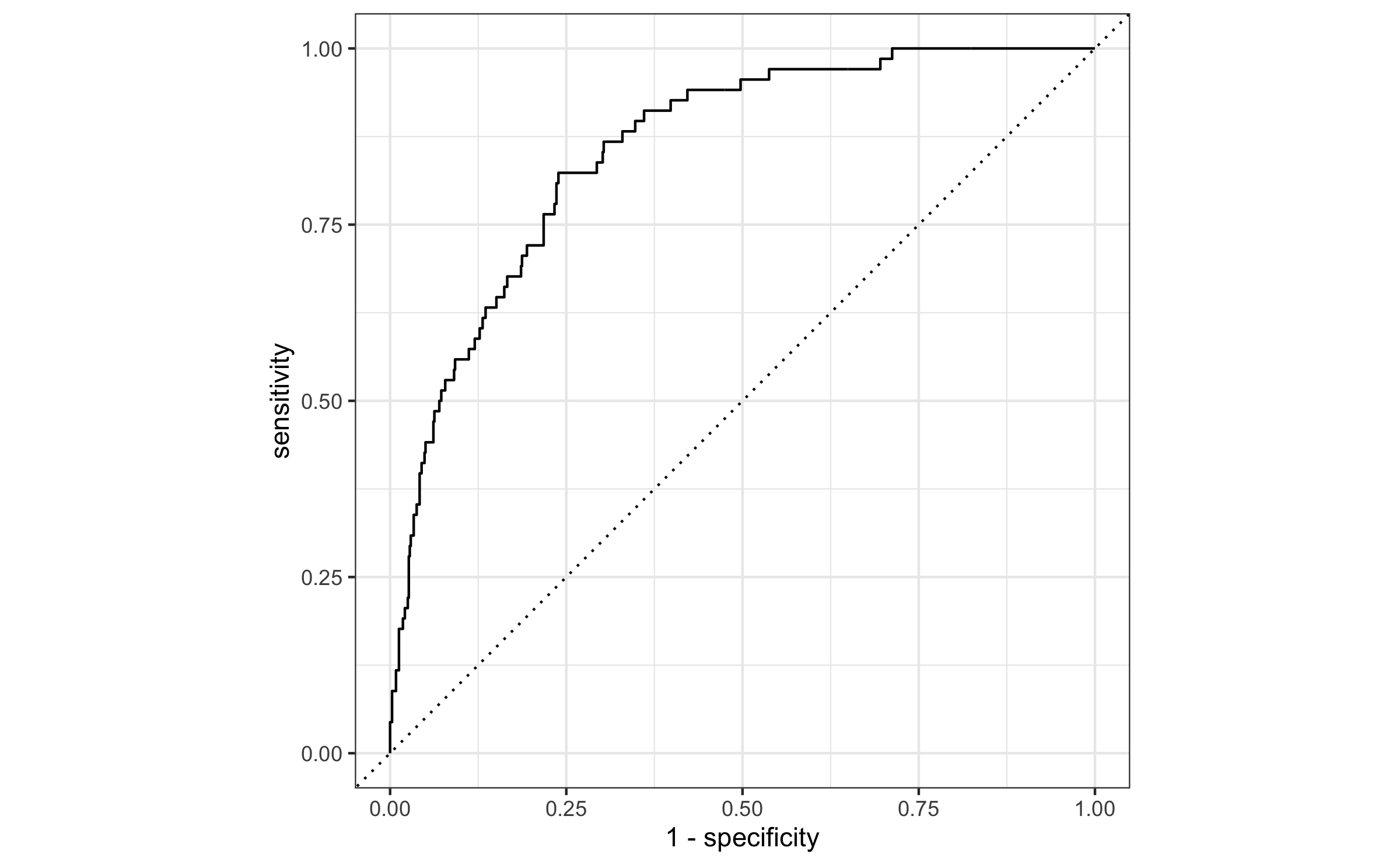
22 / 26
Cutoff probability: 0.5
Suppose we decide to label an email as spam if the model predicts the probability of spam to be more than 0.5.
| Email is not spam | Email is spam | |
|---|---|---|
| Email labelled not spam | 710 | 60 |
| Email labelled spam | 6 | 8 |
| NA | 1 | NA |
cutoff_prob <- 0.5email_pred %>% mutate( spam = if_else(spam == 1, "Email is spam", "Email is not spam"), spam_pred = if_else(.pred_1 > cutoff_prob, "Email labelled spam", "Email labelled not spam") ) %>% count(spam_pred, spam) %>% pivot_wider(names_from = spam, values_from = n) %>% kable(col.names = c("", "Email is not spam", "Email is spam"))24 / 26
Cutoff probability: 0.25
Suppose we decide to label an email as spam if the model predicts the probability of spam to be more than 0.25.
| Email is not spam | Email is spam | |
|---|---|---|
| Email labelled not spam | 665 | 34 |
| Email labelled spam | 51 | 34 |
| NA | 1 | NA |
cutoff_prob <- 0.25email_pred %>% mutate( spam = if_else(spam == 1, "Email is spam", "Email is not spam"), spam_pred = if_else(.pred_1 > cutoff_prob, "Email labelled spam", "Email labelled not spam") ) %>% count(spam_pred, spam) %>% pivot_wider(names_from = spam, values_from = n) %>% kable(col.names = c("", "Email is not spam", "Email is spam"))25 / 26
Cutoff probability: 0.75
Suppose we decide to label an email as spam if the model predicts the probability of spam to be more than 0.75.
| Email is not spam | Email is spam | |
|---|---|---|
| Email labelled not spam | 714 | 65 |
| Email labelled spam | 2 | 3 |
| NA | 1 | NA |
cutoff_prob <- 0.75email_pred %>% mutate( spam = if_else(spam == 1, "Email is spam", "Email is not spam"), spam_pred = if_else(.pred_1 > cutoff_prob, "Email labelled spam", "Email labelled not spam") ) %>% count(spam_pred, spam) %>% pivot_wider(names_from = spam, values_from = n) %>% kable(col.names = c("", "Email is not spam", "Email is spam"))26 / 26