Cross validation

Data Science in a Box

datasciencebox.org

1 / 33

Data and exploration

2 / 33

3 / 33

Data

office_ratings <- read_csv("data/office_ratings.csv")
office_ratings

## # A tibble: 188 × 6
##   season episode title         imdb_rating total_votes air_date  
##    <dbl>   <dbl> <chr>               <dbl>       <dbl> <date>    
## 1      1       1 Pilot                 7.6        3706 2005-03-24
## 2      1       2 Diversity Day         8.3        3566 2005-03-29
## 3      1       3 Health Care           7.9        2983 2005-04-05
## 4      1       4 The Alliance          8.1        2886 2005-04-12
## 5      1       5 Basketball            8.4        3179 2005-04-19
## 6      1       6 Hot Girl              7.8        2852 2005-04-26
## # … with 182 more rows

Source: The data come from data.world, by way of TidyTuesday.

4 / 33

IMDB ratings

ggplot(office_ratings, aes(x = imdb_rating)) +
  geom_histogram(binwidth = 0.25) +
  labs(
    title = "The Office ratings",
    x = "IMDB Rating"
  )

5 / 33

IMDB ratings vs. number of votes

ggplot(office_ratings, aes(x = total_votes, y = imdb_rating, color = season)) +
  geom_jitter(alpha = 0.7) +
  labs(
    title = "The Office ratings",
    x = "Total votes",
    y = "IMDB Rating",
    color = "Season"
  )

6 / 33

Outliers

ggplot(office_ratings, aes(x = total_votes, y = imdb_rating)) +
  geom_jitter() +
  gghighlight(total_votes > 4000, label_key = title) +
  labs(
    title = "The Office ratings",
    x = "Total votes",
    y = "IMDB Rating"
  )

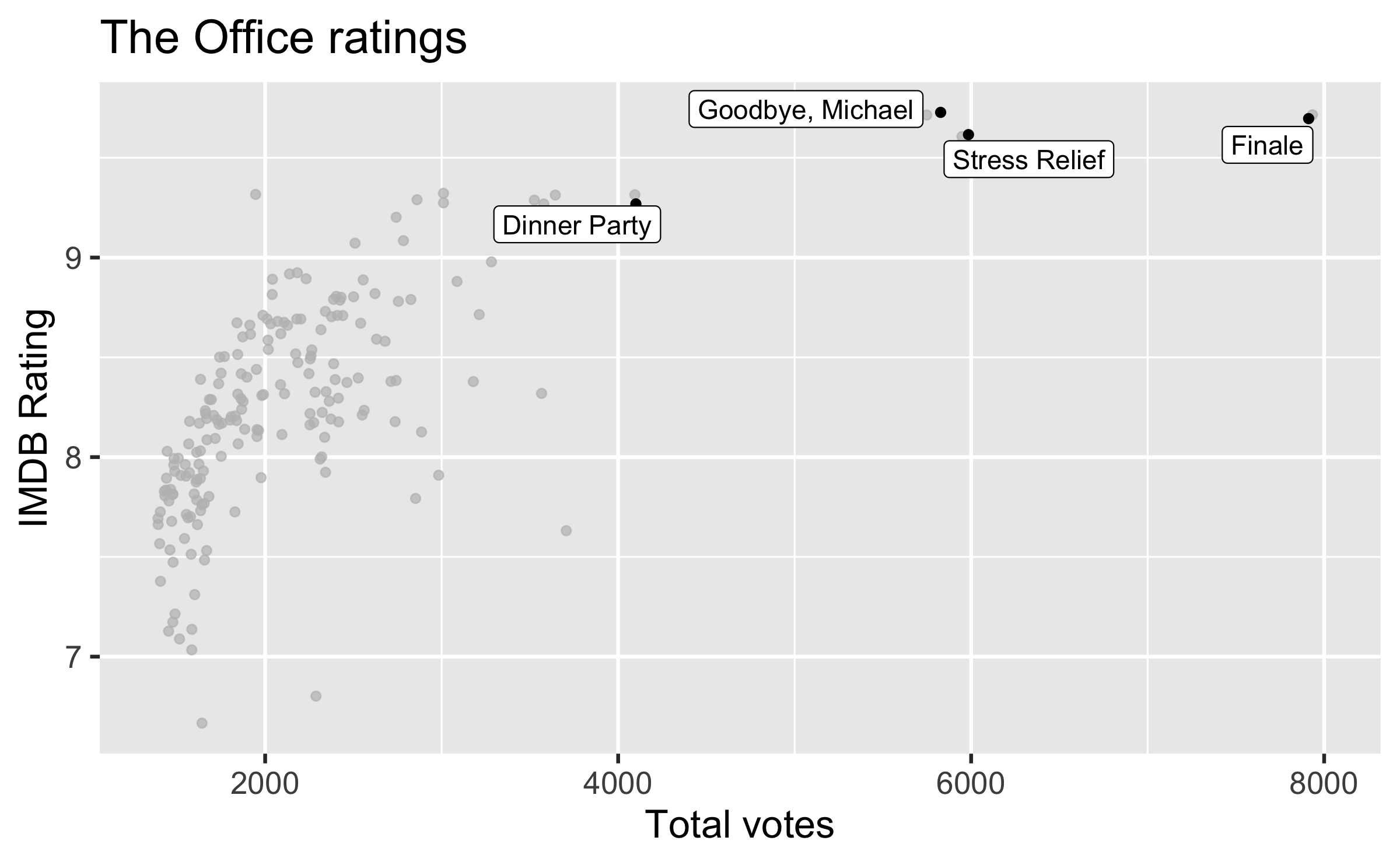
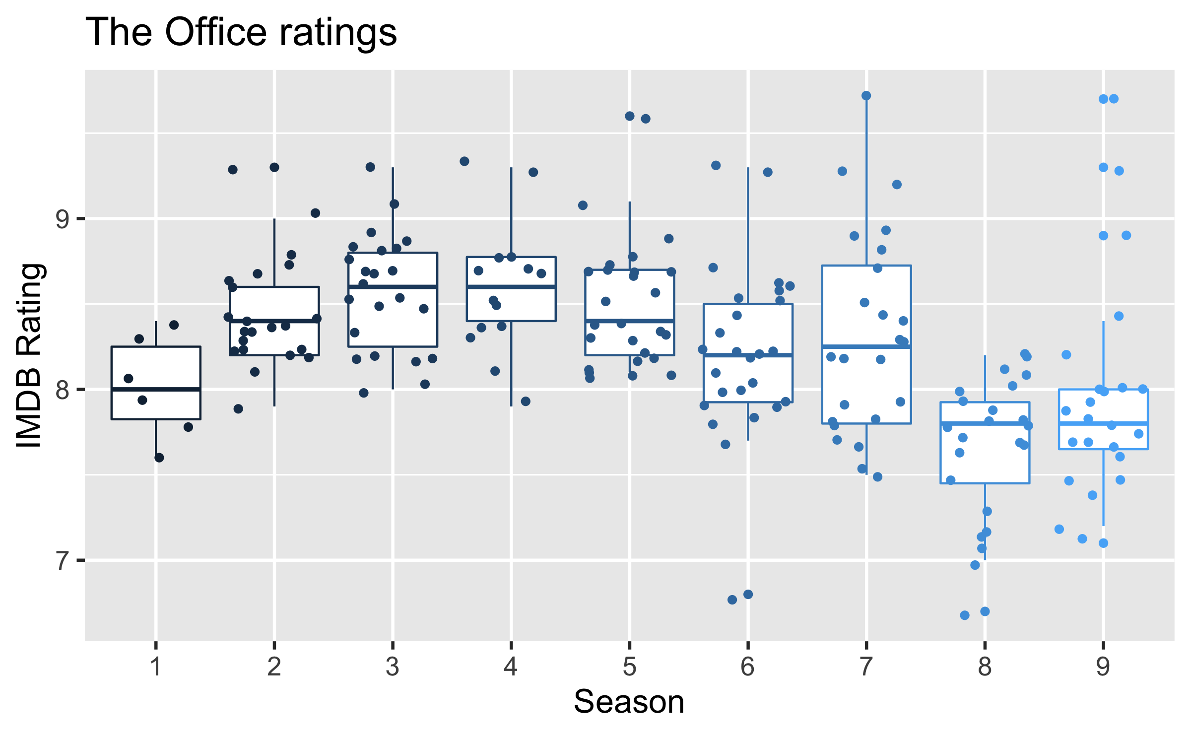
If you like the Dinner Party episode, I highly recommend this "oral history" of the episode published on Rolling Stone magazine.

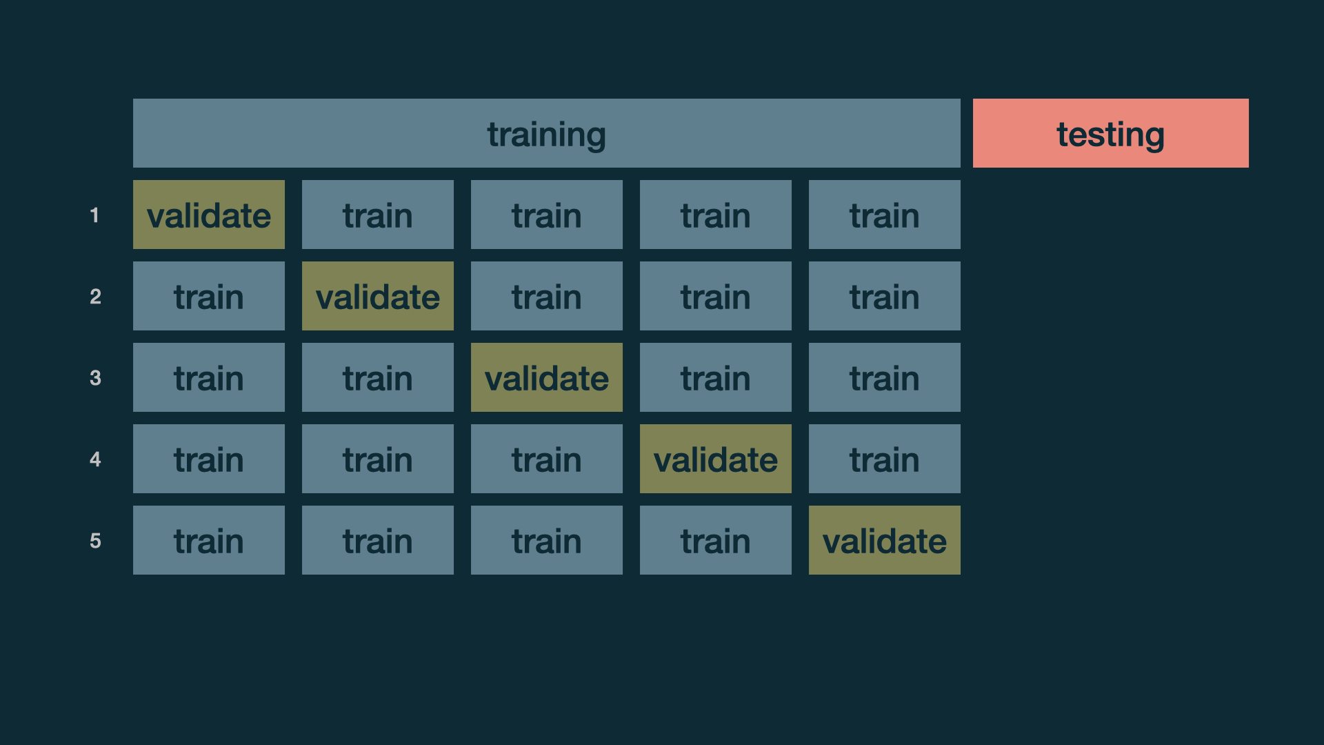
7 / 33

IMDB ratings vs. seasons

ggplot(office_ratings, aes(x = factor(season), y = imdb_rating, color = season)) +
  geom_boxplot() +
  geom_jitter() +
  guides(color = "none") +
  labs(
    title = "The Office ratings",
    x = "Season",
    y = "IMDB Rating"
  )

8 / 33

Modeling

9 / 33

Train / test

Create an initial split

set.seed(1122)
office_split <- initial_split(office_ratings) # prop = 3/4 by default

10 / 33

Train / test

Create an initial split

set.seed(1122)
office_split <- initial_split(office_ratings) # prop = 3/4 by default

Save training data

office_train <- training(office_split)
dim(office_train)

## [1] 141   6

10 / 33

Train / test

Create an initial split

set.seed(1122)
office_split <- initial_split(office_ratings) # prop = 3/4 by default

Save training data

office_train <- training(office_split)
dim(office_train)

## [1] 141   6

Save testing data

office_test  <- testing(office_split)
dim(office_test)

## [1] 47  6

10 / 33

Specify model

office_mod <- linear_reg() %>%
  set_engine("lm")
office_mod

## Linear Regression Model Specification (regression)
## 
## Computational engine: lm

11 / 33

datasciencebox.org

Build recipeCode
Output
office_rec <- recipe(imdb_rating ~ ., data = office_train) %>%
  # title isn't a predictor, but keep around to ID
  update_role(title, new_role = "ID") %>%
  # extract month of air_date
  step_date(air_date, features = "month") %>%
  step_rm(air_date) %>%
  # make dummy variables of month 
  step_dummy(contains("month")) %>%
  # remove zero variance predictors
  step_zv(all_predictors())
office_rec

## Recipe
## 
## Inputs:
## 
##       role #variables
##         ID          1
##    outcome          1
##  predictor          4
## 
## Operations:
## 
## Date features from air_date
## Variables removed air_date
## Dummy variables from contains("month")
## Zero variance filter on all_predictors()
12 / 33

Build workflow

office_wflow <- workflow() %>%
  add_model(office_mod) %>%
  add_recipe(office_rec)

office_wflow

## ══ Workflow ═════════════════════════════════════════════════════
## Preprocessor: Recipe
## Model: linear_reg()
## 
## ── Preprocessor ─────────────────────────────────────────────────
## 4 Recipe Steps
## 
## • step_date()
## • step_rm()
## • step_dummy()
## • step_zv()
## 
## ── Model ────────────────────────────────────────────────────────
## Linear Regression Model Specification (regression)
## 
## Computational engine: lm

13 / 33

Fit model

office_fit <- office_wflow %>%
  fit(data = office_train)

tidy(office_fit) %>%
  print(n = 12)

## # A tibble: 12 × 5
##    term                estimate std.error statistic  p.value
##    <chr>                  <dbl>     <dbl>     <dbl>    <dbl>
##  1 (Intercept)         7.23     0.205        35.4   3.14e-68
##  2 season             -0.0499   0.0157       -3.18  1.86e- 3
##  3 episode             0.0353   0.0101        3.50  6.44e- 4
##  4 total_votes         0.000352 0.0000448     7.85  1.39e-12
##  5 air_date_month_Feb  0.0242   0.147         0.165 8.69e- 1
##  6 air_date_month_Mar -0.145    0.144        -1.01  3.16e- 1
##  7 air_date_month_Apr -0.106    0.140        -0.759 4.49e- 1
##  8 air_date_month_May  0.0575   0.175         0.329 7.43e- 1
##  9 air_date_month_Sep  0.440    0.191         2.30  2.30e- 2
## 10 air_date_month_Oct  0.321    0.150         2.13  3.50e- 2
## 11 air_date_month_Nov  0.237    0.138         1.72  8.81e- 2
## 12 air_date_month_Dec  0.443    0.190         2.34  2.09e- 2

14 / 33

Evaluate model

15 / 33

Make predictions for training data

office_train_pred <- predict(office_fit, office_train) %>%
  bind_cols(office_train %>% select(imdb_rating, title))
office_train_pred

## # A tibble: 141 × 3
##   .pred imdb_rating title            
##   <dbl>       <dbl> <chr>            
## 1  7.90         8.1 Garden Party     
## 2  8.43         7.9 The Chump        
## 3  7.81         7.1 Here Comes Treble
## 4  7.94         6.7 Get the Girl     
## 5  7.92         7.9 Tallahassee      
## 6  8.29         7.7 The Inner Circle 
## # … with 135 more rows

16 / 33

R-squared

Percentage of variability in the IMDB ratings explained by the model

rsq(office_train_pred, truth = imdb_rating, estimate = .pred)

## # A tibble: 1 × 3
##   .metric .estimator .estimate
##   <chr>   <chr>          <dbl>
## 1 rsq     standard       0.500

17 / 33

R-squared

Percentage of variability in the IMDB ratings explained by the model

rsq(office_train_pred, truth = imdb_rating, estimate = .pred)

## # A tibble: 1 × 3
##   .metric .estimator .estimate
##   <chr>   <chr>          <dbl>
## 1 rsq     standard       0.500

Are models with high or low $R^{2}$ more preferable?

17 / 33

RMSE

An alternative model performance statistic: root mean square error

$R M S E = \sqrt{\frac{\sum_{i = 1}^{n} (y_{i} - {\hat{y}}_{i})^{2}}{n}}$

18 / 33

RMSE

An alternative model performance statistic: root mean square error

$R M S E = \sqrt{\frac{\sum_{i = 1}^{n} (y_{i} - {\hat{y}}_{i})^{2}}{n}}$

rmse(office_train_pred, truth = imdb_rating, estimate = .pred)

## # A tibble: 1 × 3
##   .metric .estimator .estimate
##   <chr>   <chr>          <dbl>
## 1 rmse    standard       0.373

18 / 33

RMSE

An alternative model performance statistic: root mean square error

$R M S E = \sqrt{\frac{\sum_{i = 1}^{n} (y_{i} - {\hat{y}}_{i})^{2}}{n}}$

rmse(office_train_pred, truth = imdb_rating, estimate = .pred)

## # A tibble: 1 × 3
##   .metric .estimator .estimate
##   <chr>   <chr>          <dbl>
## 1 rmse    standard       0.373

Are models with high or low RMSE are more preferable?

18 / 33

Interpreting RMSE

Is this RMSE considered low or high?

rmse(office_train_pred, truth = imdb_rating, estimate = .pred)

## # A tibble: 1 × 3
##   .metric .estimator .estimate
##   <chr>   <chr>          <dbl>
## 1 rmse    standard       0.373

19 / 33

Interpreting RMSE

Is this RMSE considered low or high?

rmse(office_train_pred, truth = imdb_rating, estimate = .pred)

## # A tibble: 1 × 3
##   .metric .estimator .estimate
##   <chr>   <chr>          <dbl>
## 1 rmse    standard       0.373

office_train %>%
  summarise(min = min(imdb_rating), max = max(imdb_rating))

## # A tibble: 1 × 2
##     min   max
##   <dbl> <dbl>
## 1   6.7   9.7

19 / 33

but, really, who cares about predictions on training data?

20 / 33

Make predictions for testing data

office_test_pred <- predict(office_fit, office_test) %>%
  bind_cols(office_test %>% select(imdb_rating, title))
office_test_pred

## # A tibble: 47 × 3
##   .pred imdb_rating title          
##   <dbl>       <dbl> <chr>          
## 1  8.52         8.4 Office Olympics
## 2  8.54         8.6 The Client     
## 3  8.90         8.8 Christmas Party
## 4  8.71         9   The Injury     
## 5  8.50         8.2 Boys and Girls 
## 6  8.46         8.4 Dwight's Speech
## # … with 41 more rows

21 / 33

Evaluate performance on testing data

RMSE of model fit to testing data

rmse(office_test_pred, truth = imdb_rating, estimate = .pred)

## # A tibble: 1 × 3
##   .metric .estimator .estimate
##   <chr>   <chr>          <dbl>
## 1 rmse    standard       0.386

$R^{2}$ of model fit to testing data

rsq(office_test_pred, truth = imdb_rating, estimate = .pred)

## # A tibble: 1 × 3
##   .metric .estimator .estimate
##   <chr>   <chr>          <dbl>
## 1 rsq     standard       0.556

22 / 33

Training vs. testing

metric	train	test	comparison
RMSE	0.373	0.386	RMSE lower for training
R-squared	0.500	0.556	R-squared higher for training

23 / 33

Evaluating performance on training data

The training set does not have the capacity to be a good arbiter of performance.

24 / 33

Evaluating performance on training data

The training set does not have the capacity to be a good arbiter of performance.
It is not an independent piece of information; predicting the training set can only reflect what the model already knows.

24 / 33

Evaluating performance on training data

The training set does not have the capacity to be a good arbiter of performance.
It is not an independent piece of information; predicting the training set can only reflect what the model already knows.
Suppose you give a class a test, then give them the answers, then provide the same test. The student scores on the second test do not accurately reflect what they know about the subject; these scores would probably be higher than their results on the first test.

Source: tidymodels.org

24 / 33

Cross validation

25 / 33

Cross validation

More specifically, v-fold cross validation:

Shuffle your data v partitions
Use 1 partition for validation, and the remaining v-1 partitions for training
Repeat v times

You might also heard of this referred to as k-fold cross validation.

26 / 33

Cross validation

27 / 33

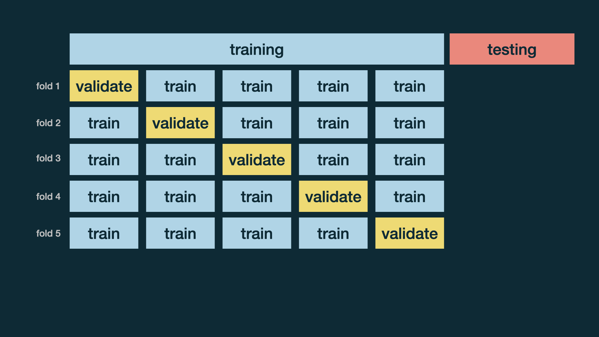
Split data into folds

set.seed(345)
folds <- vfold_cv(office_train, v = 5)
folds

## #  5-fold cross-validation 
## # A tibble: 5 × 2
##   splits           id   
##   <list>           <chr>
## 1 <split [112/29]> Fold1
## 2 <split [113/28]> Fold2
## 3 <split [113/28]> Fold3
## 4 <split [113/28]> Fold4
## 5 <split [113/28]> Fold5

28 / 33

Fit resamples

set.seed(456)
office_fit_rs <- office_wflow %>%
  fit_resamples(folds)
office_fit_rs

## # Resampling results
## # 5-fold cross-validation 
## # A tibble: 5 × 4
##   splits           id    .metrics         .notes          
##   <list>           <chr> <list>           <list>          
## 1 <split [112/29]> Fold1 <tibble [2 × 4]> <tibble [0 × 3]>
## 2 <split [113/28]> Fold2 <tibble [2 × 4]> <tibble [0 × 3]>
## 3 <split [113/28]> Fold3 <tibble [2 × 4]> <tibble [0 × 3]>
## 4 <split [113/28]> Fold4 <tibble [2 × 4]> <tibble [0 × 3]>
## 5 <split [113/28]> Fold5 <tibble [2 × 4]> <tibble [0 × 3]>

29 / 33

Collect CV metrics

collect_metrics(office_fit_rs)

## # A tibble: 2 × 6
##   .metric .estimator  mean     n std_err .config             
##   <chr>   <chr>      <dbl> <int>   <dbl> <chr>               
## 1 rmse    standard   0.403     5  0.0336 Preprocessor1_Model1
## 2 rsq     standard   0.413     5  0.0727 Preprocessor1_Model1

30 / 33

Deeper look into CV metrics

collect_metrics(office_fit_rs, summarize = FALSE) %>%
  print(n = 10)

## # A tibble: 10 × 5
##    id    .metric .estimator .estimate .config             
##    <chr> <chr>   <chr>          <dbl> <chr>               
##  1 Fold1 rmse    standard       0.430 Preprocessor1_Model1
##  2 Fold1 rsq     standard       0.134 Preprocessor1_Model1
##  3 Fold2 rmse    standard       0.368 Preprocessor1_Model1
##  4 Fold2 rsq     standard       0.496 Preprocessor1_Model1
##  5 Fold3 rmse    standard       0.452 Preprocessor1_Model1
##  6 Fold3 rsq     standard       0.501 Preprocessor1_Model1
##  7 Fold4 rmse    standard       0.289 Preprocessor1_Model1
##  8 Fold4 rsq     standard       0.529 Preprocessor1_Model1
##  9 Fold5 rmse    standard       0.475 Preprocessor1_Model1
## 10 Fold5 rsq     standard       0.403 Preprocessor1_Model1

Fold	RMSE	R-squared
Fold1	0.430	0.134
Fold2	0.368	0.496
Fold3	0.452	0.501
Fold4	0.289	0.529
Fold5	0.475	0.403

31 / 33

How does RMSE compare to y?

Cross validation RMSE stats

## # A tibble: 1 × 6
##     min   max  mean   med     sd    IQR
##   <dbl> <dbl> <dbl> <dbl>  <dbl>  <dbl>
## 1 0.289 0.475 0.403 0.430 0.0751 0.0841

Training data IMDB score stats

## # A tibble: 1 × 6
##     min   max  mean   med    sd   IQR
##   <dbl> <dbl> <dbl> <dbl> <dbl> <dbl>
## 1   6.7   9.7  8.24   8.2 0.530 0.600

32 / 33

What's next?

33 / 33

Help

Keyboard shortcuts

↑, ←, Pg Up, k

Go to previous slide

↓, →, Pg Dn, Space, j

Go to next slide

Home

Go to first slide

End

Go to last slide

Number + Return

Go to specific slide

b / m / f

Toggle blackout / mirrored / fullscreen mode

Clone slideshow

Toggle presenter mode

Restart the presentation timer

?, h

Toggle this help