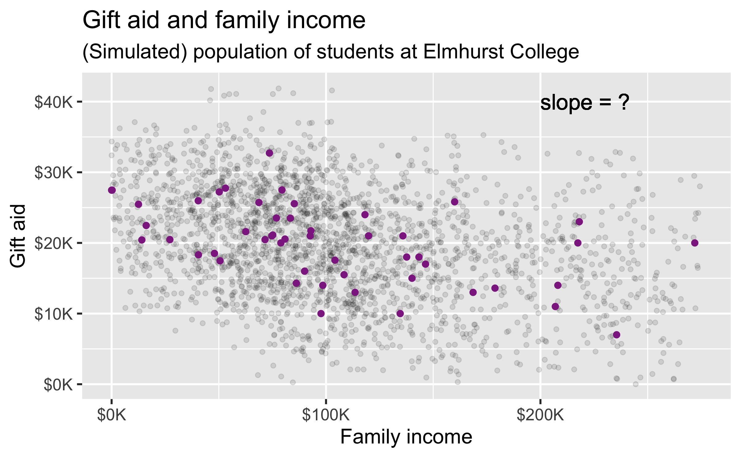
Data
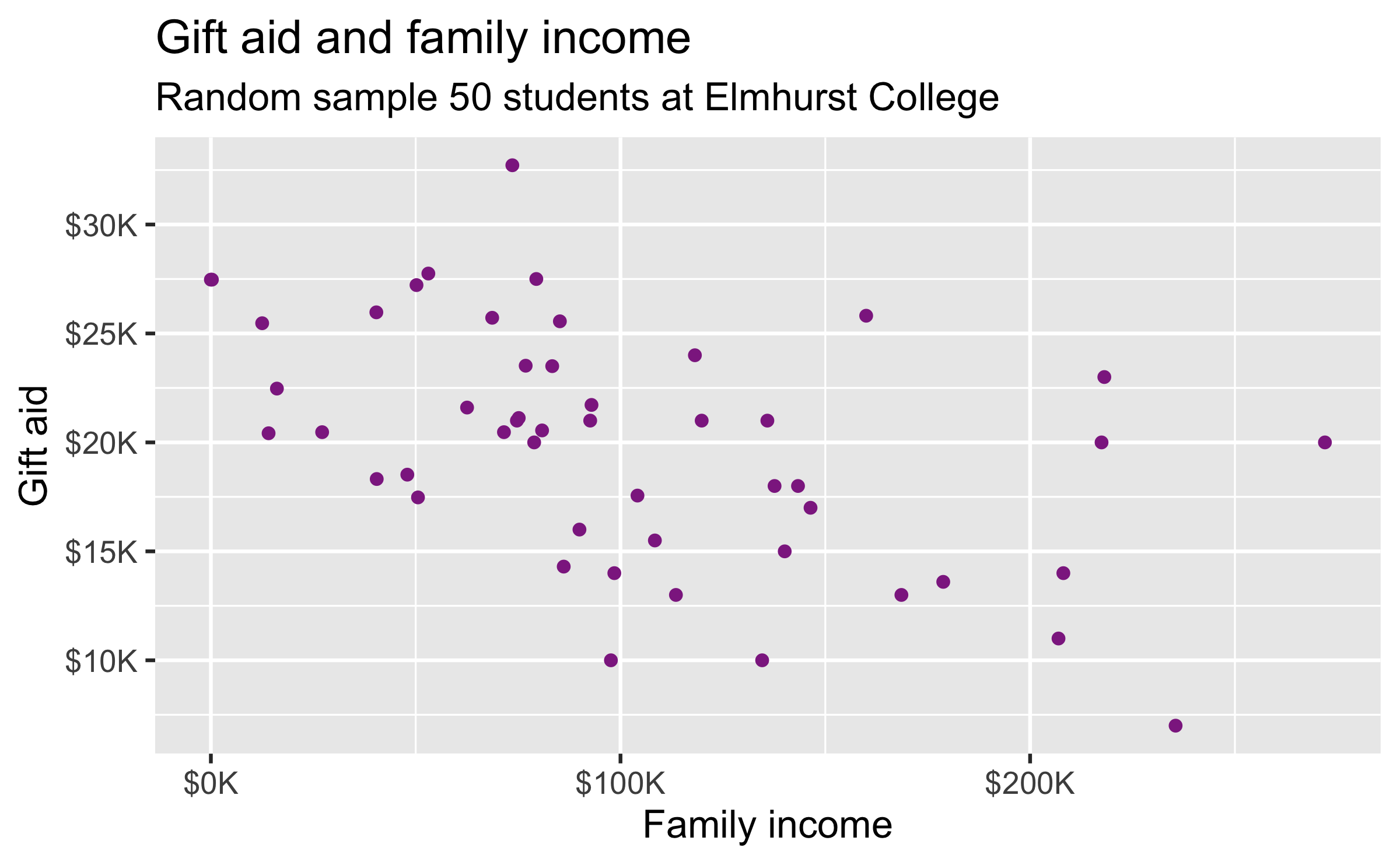
- Family income and gift aid data from a random sample of fifty students in the freshman class of Elmhurst College in Illinois, USA
- Gift aid is financial aid that does not need to be paid back, as opposed to a loan
The data come from the openintro package: elmhurst.
Linear model
linear_reg() %>% set_engine("lm") %>% fit(gift_aid ~ family_income, data = elmhurst) %>% tidy()## # A tibble: 2 × 5## term estimate std.error statistic p.value## <chr> <dbl> <dbl> <dbl> <dbl>## 1 (Intercept) 24.3 1.29 18.8 8.28e-24## 2 family_income -0.0431 0.0108 -3.98 2.29e- 4
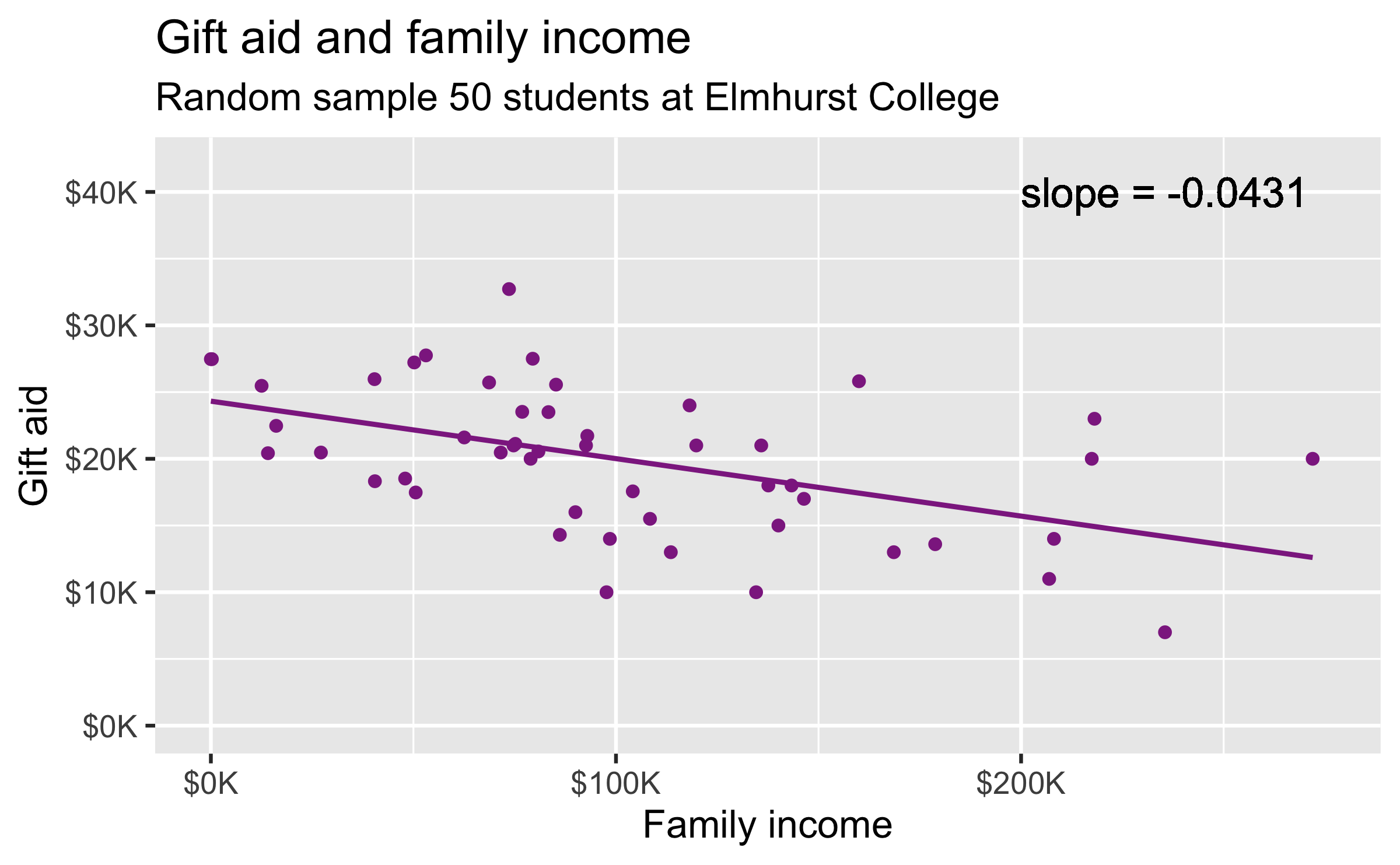
Interpreting the slope
## # A tibble: 2 × 5## term estimate std.error statistic p.value## <chr> <dbl> <dbl> <dbl> <dbl>## 1 (Intercept) 24.3 1.29 18.8 8.28e-24## 2 family_income -0.0431 0.0108 -3.98 2.29e- 4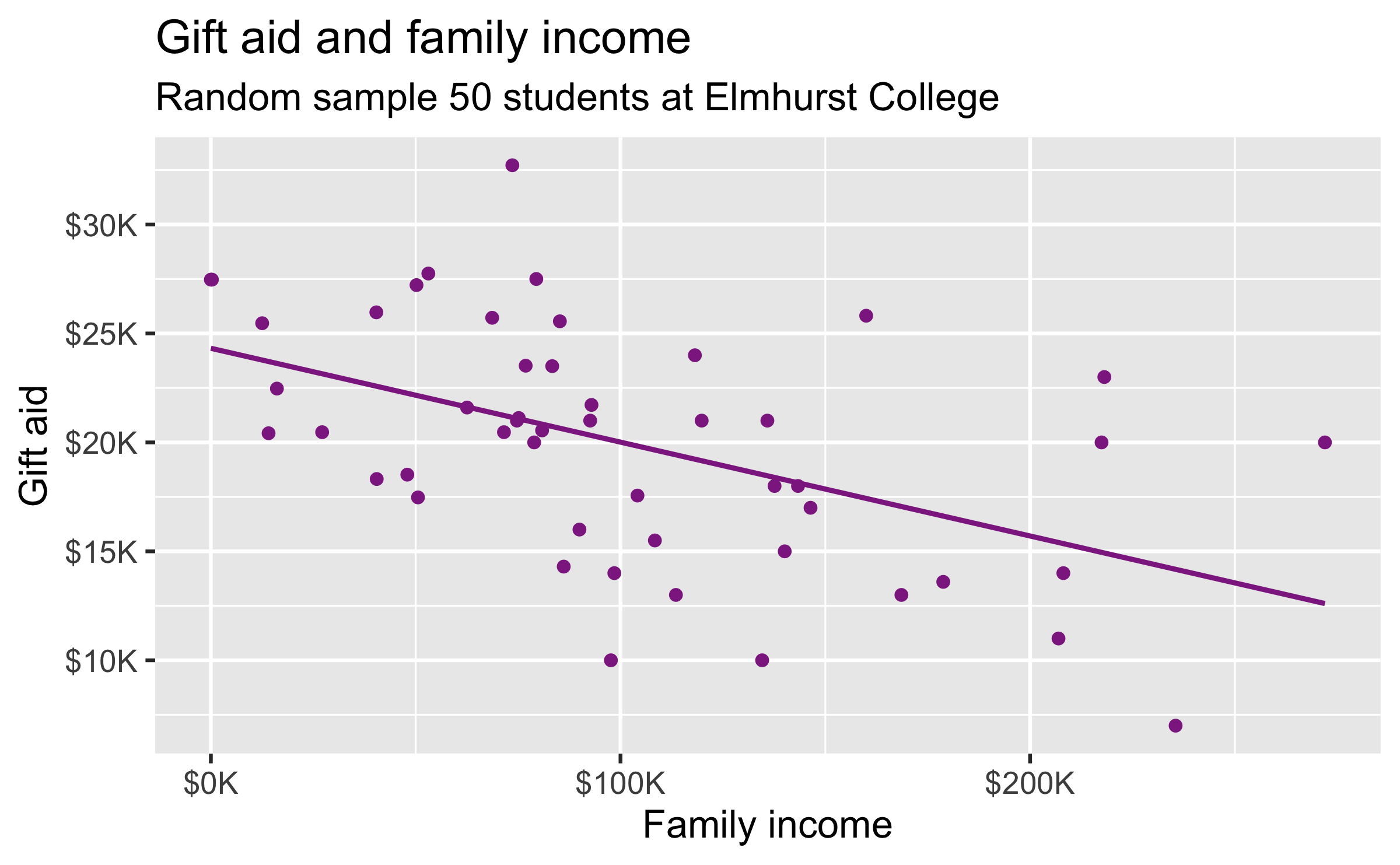
Interpreting the slope
## # A tibble: 2 × 5## term estimate std.error statistic p.value## <chr> <dbl> <dbl> <dbl> <dbl>## 1 (Intercept) 24.3 1.29 18.8 8.28e-24## 2 family_income -0.0431 0.0108 -3.98 2.29e- 4
For each additional $1,000 of family income, we would expect students to receive a net difference of 1,000 * (-0.0431) = -$43.10 in aid on average, i.e. $43.10 less in gift aid, on average.
Statistical inference
... is the process of using sample data to make conclusions about the underlying population the sample came from

If you want to catch a fish, do you prefer a spear or a net?


Observed sample
Bootstrap population
Generated assuming there are more students like the ones in the observed sample...
Bootstrap sample 1
elmhurtst_boot_1 <- elmhurst %>% slice_sample(n = 50, replace = TRUE)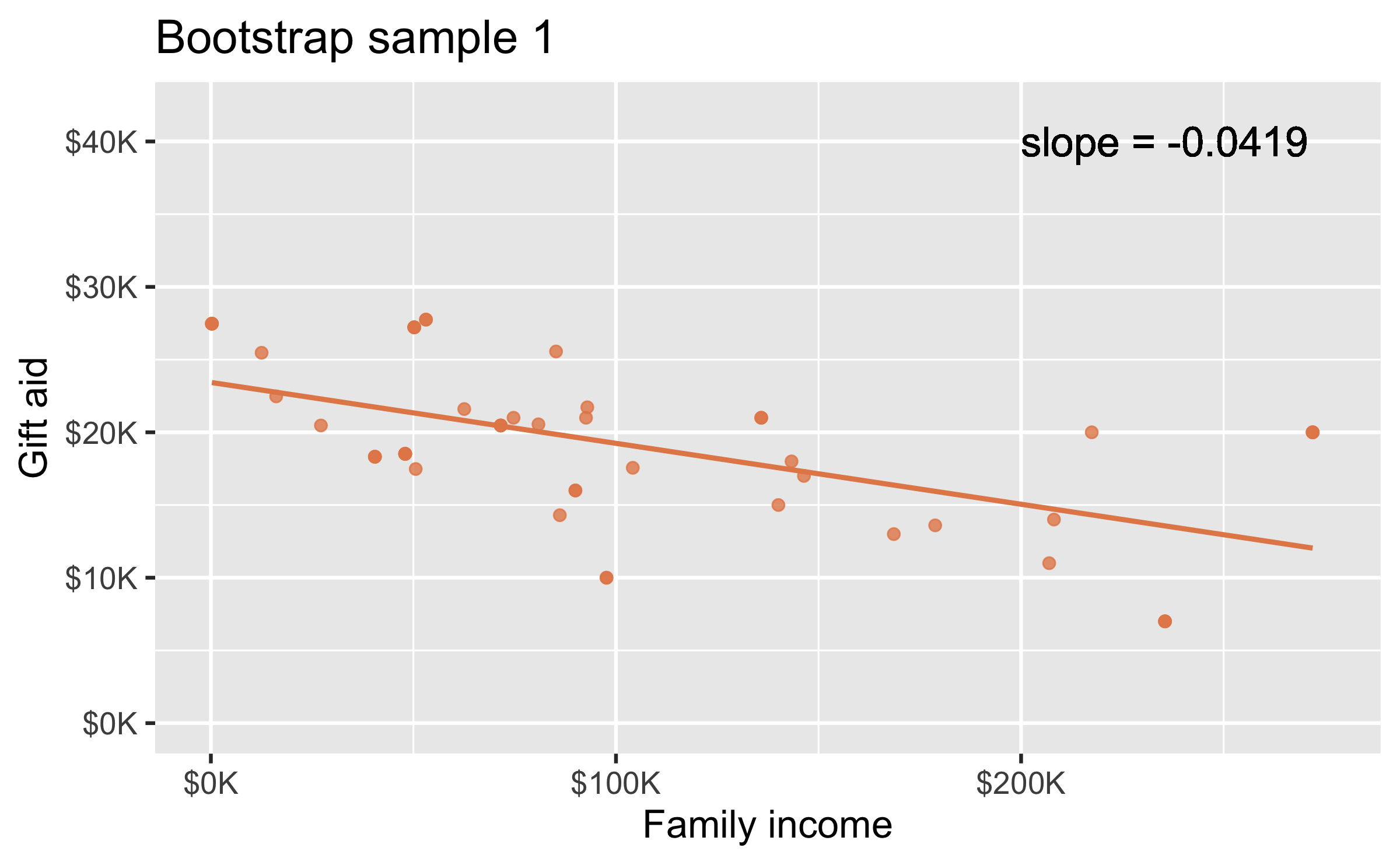
Bootstrap sample 2
elmhurtst_boot_2 <- elmhurst %>% slice_sample(n = 50, replace = TRUE)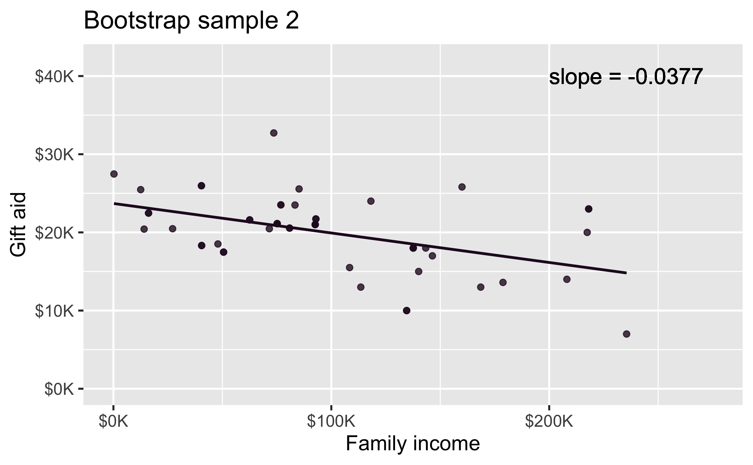
Bootstrap sample 3
elmhurtst_boot_3 <- elmhurst %>% slice_sample(n = 50, replace = TRUE)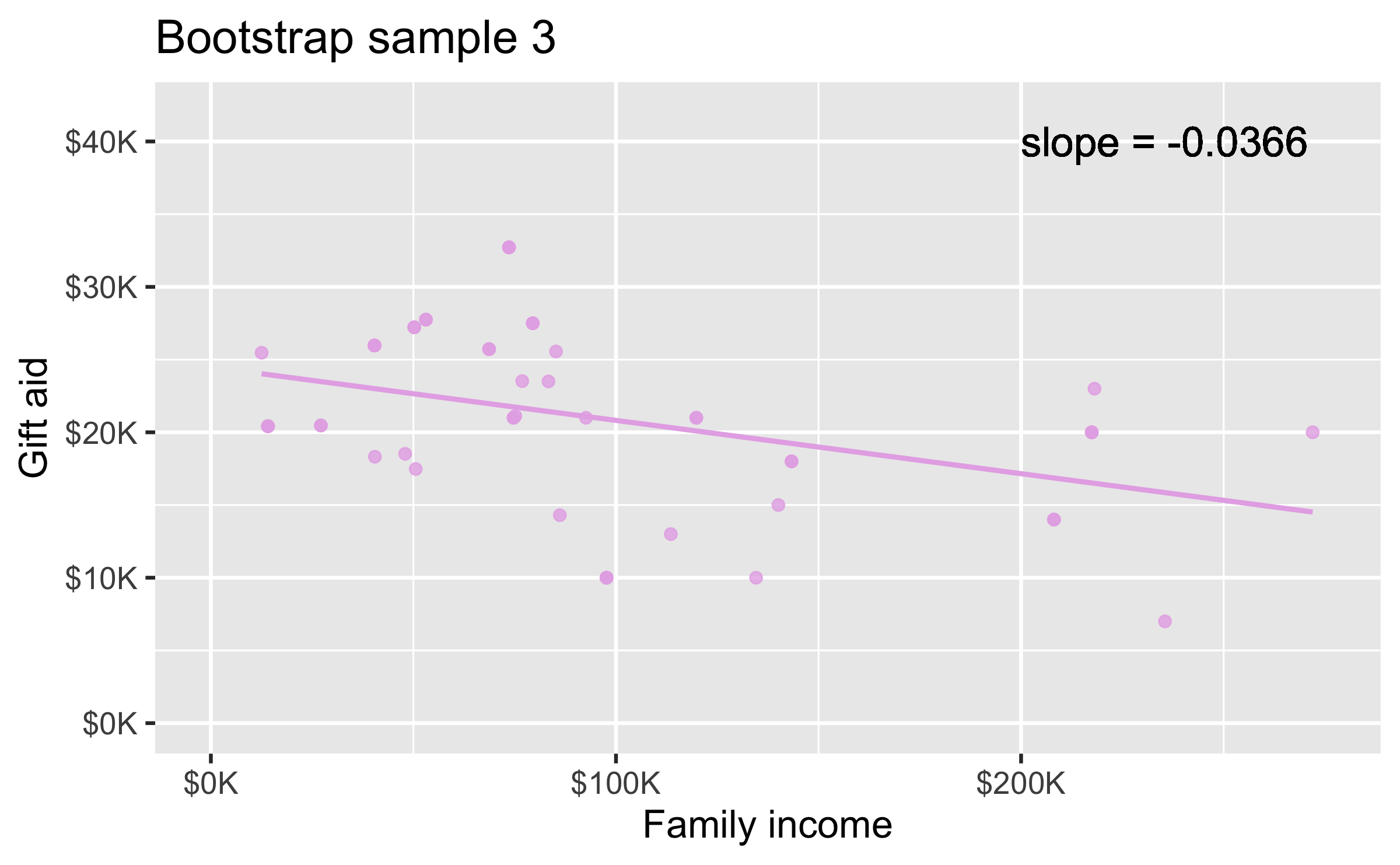
Bootstrap sample 4
elmhurtst_boot_4 <- elmhurst %>% slice_sample(n = 50, replace = TRUE)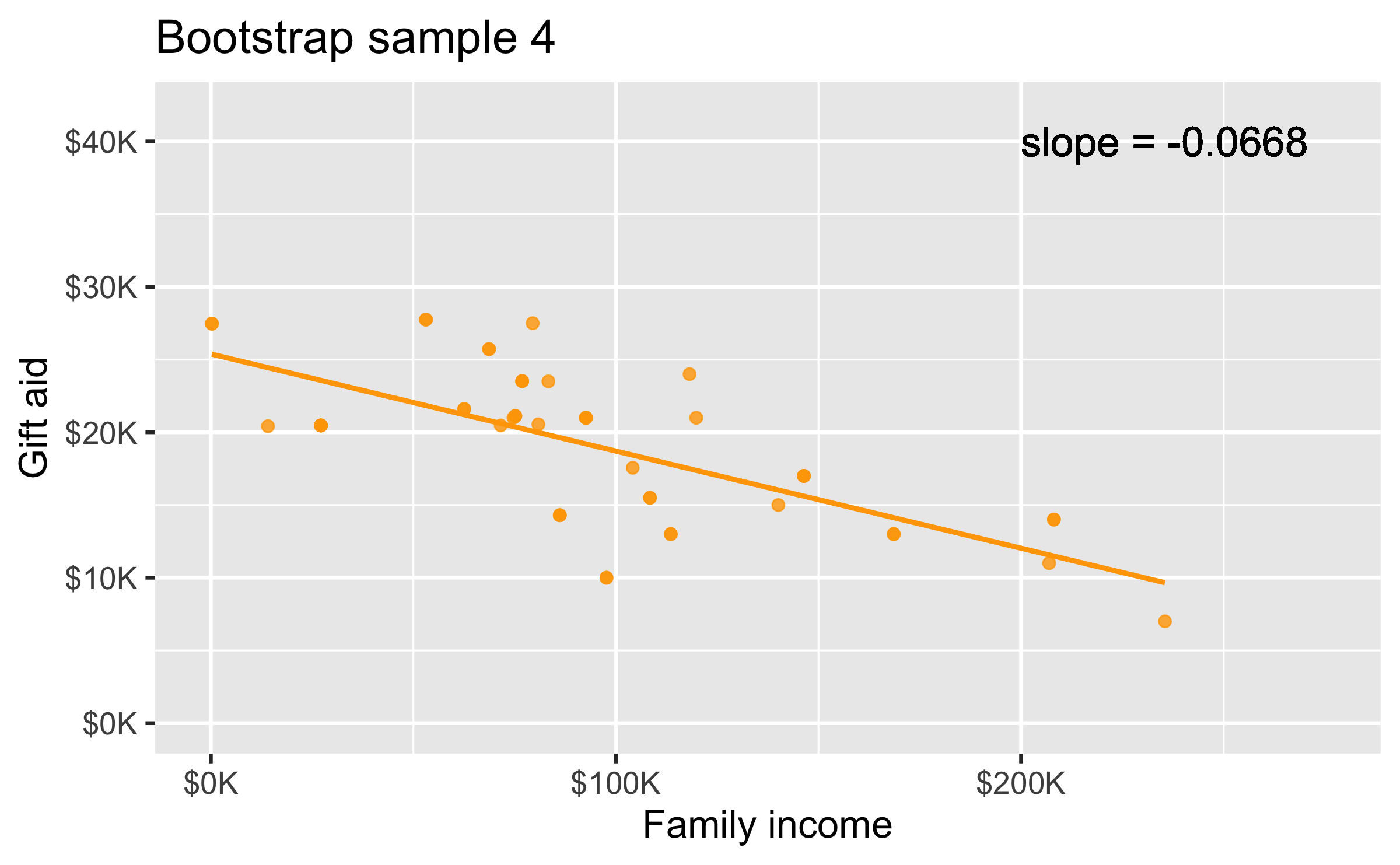
Bootstrap samples 1 - 4
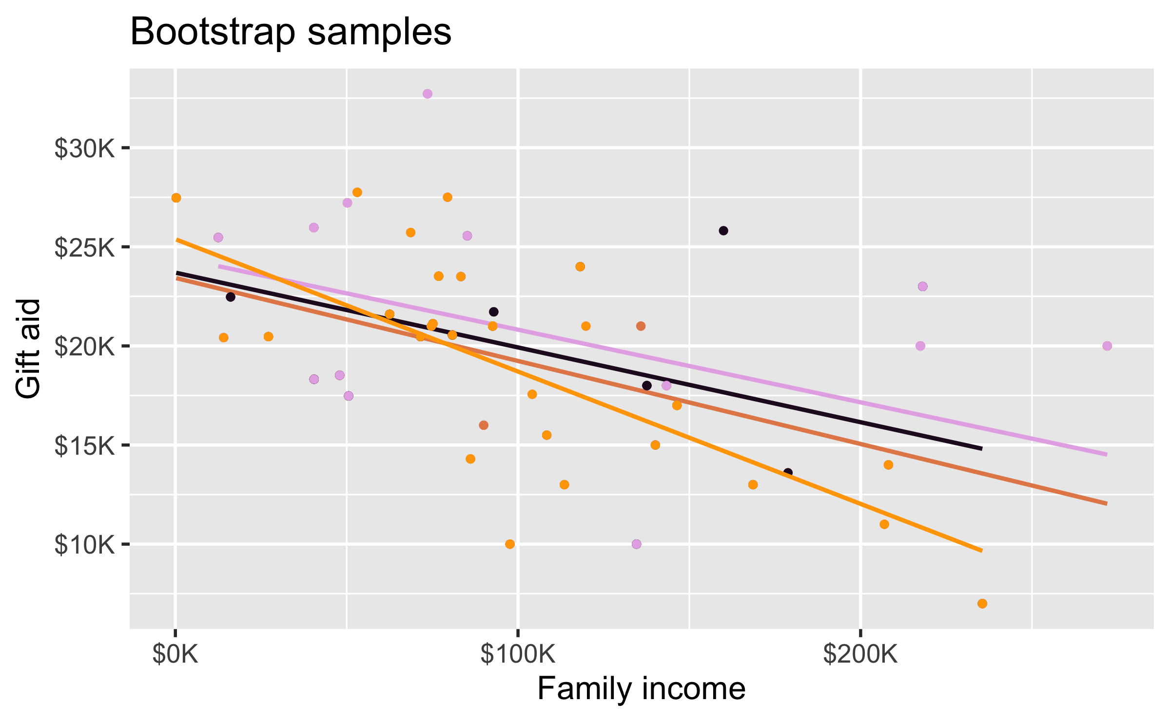
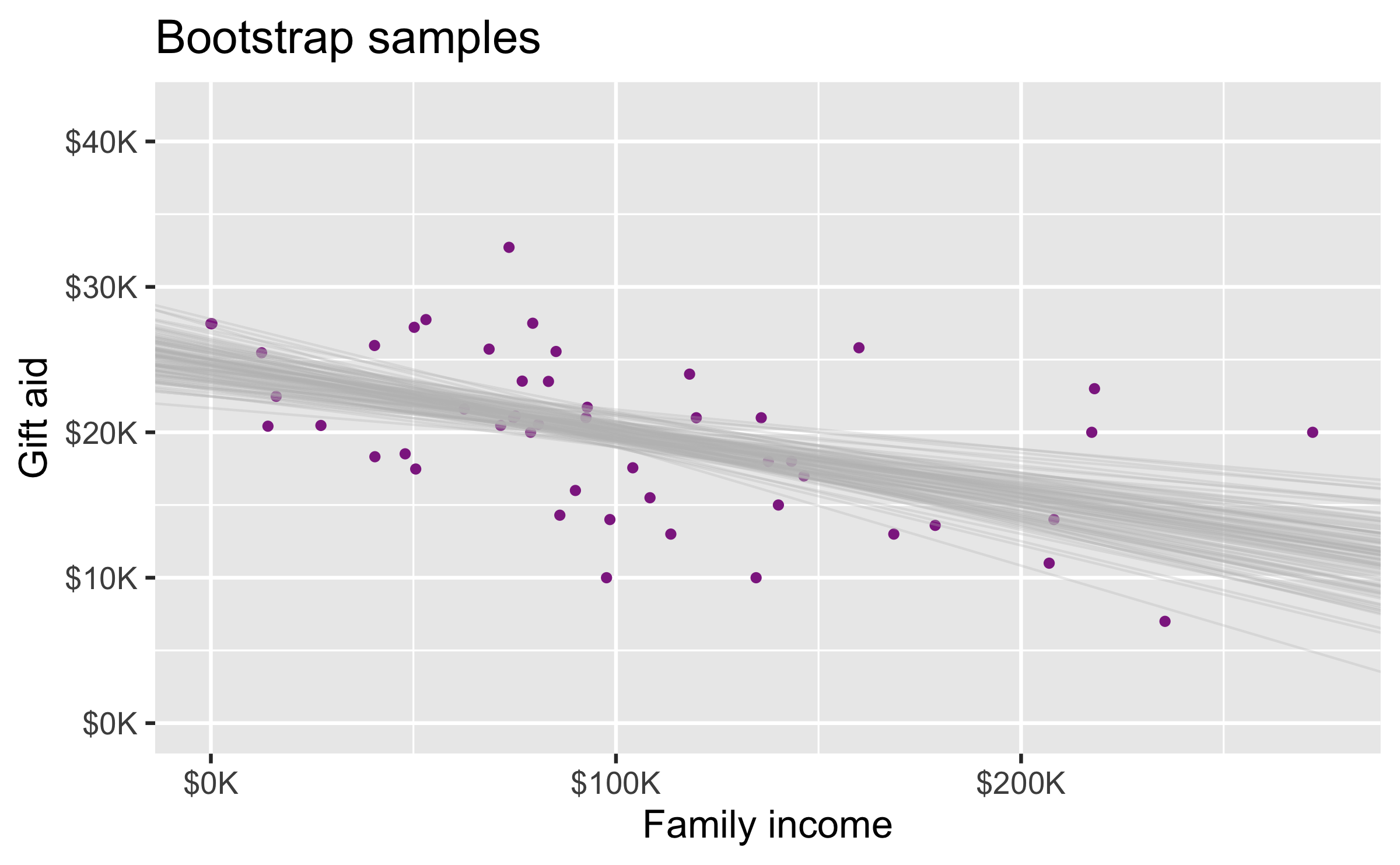
Many many samples...
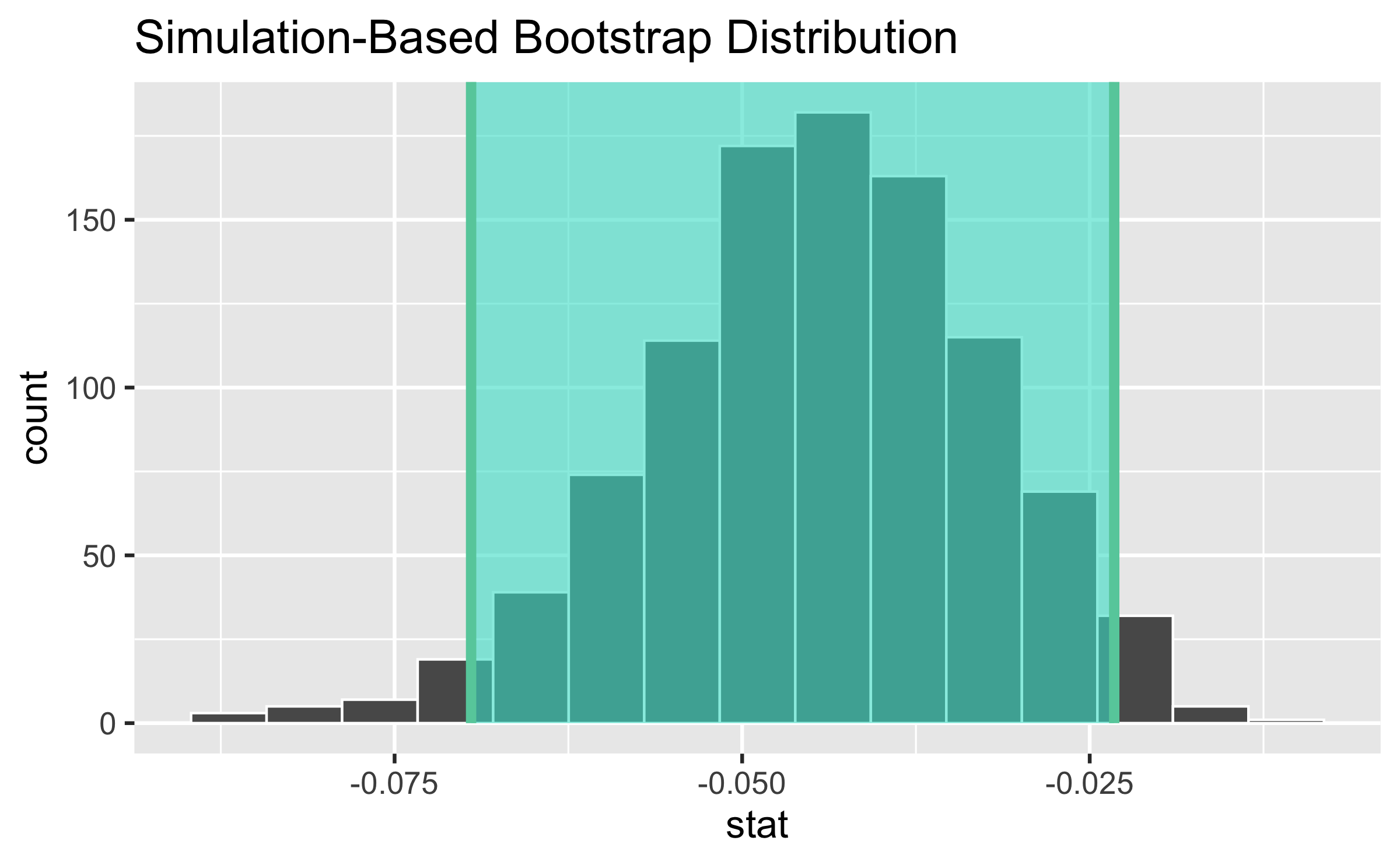
Slopes of bootstrap samples
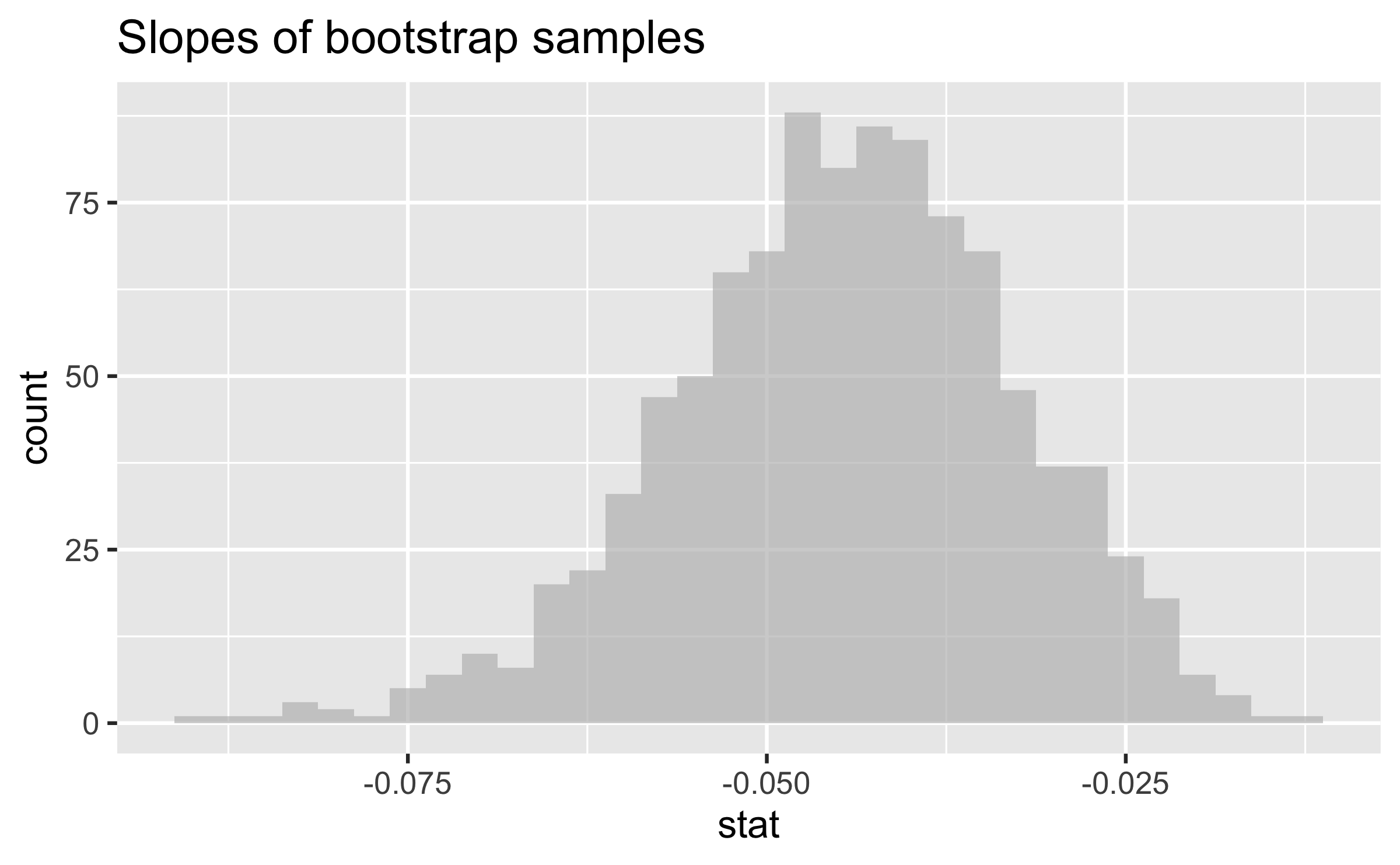
95% confidence interval