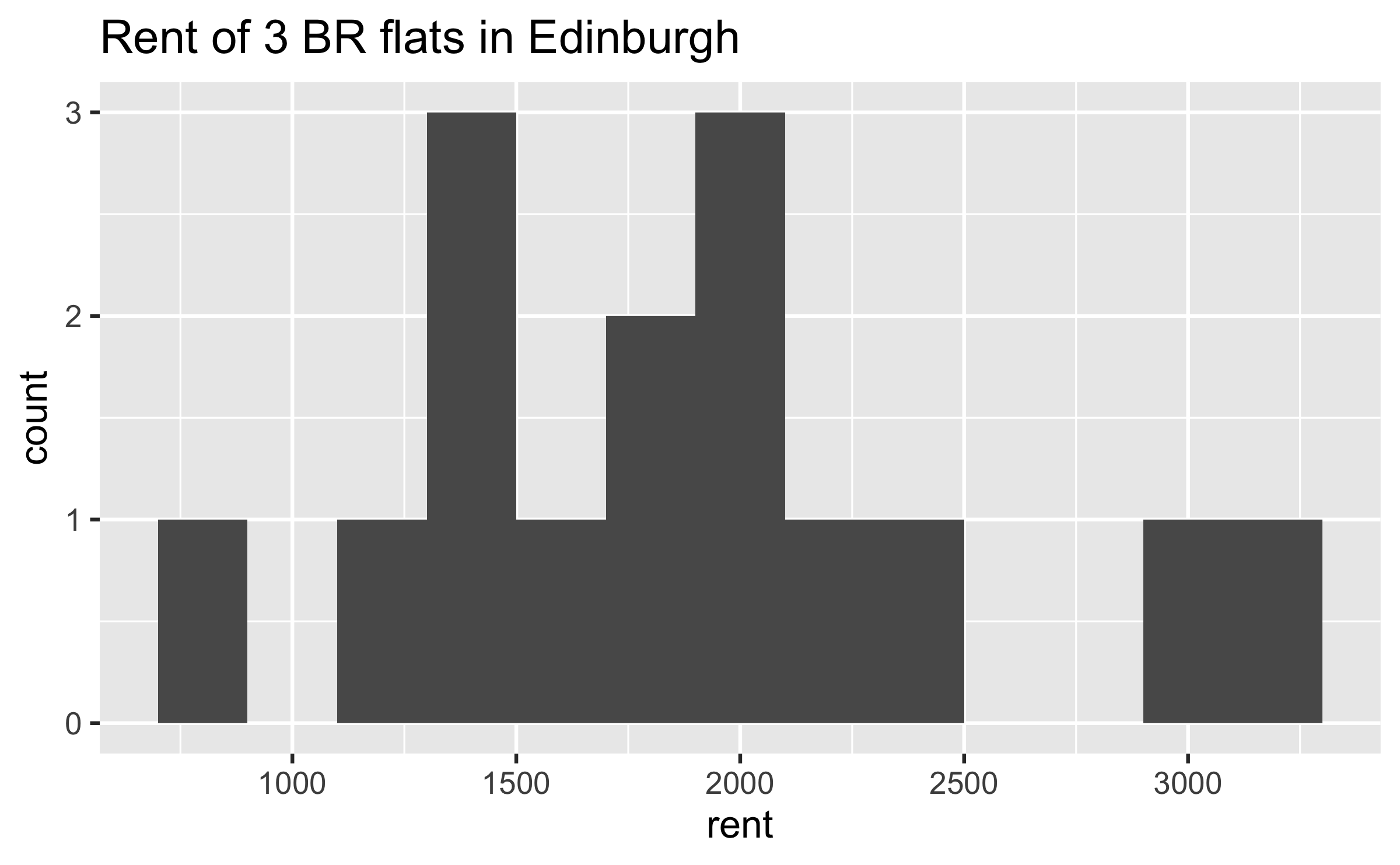
+ - 0:00:00
Notes for current slide
Notes for next slide

Bootstrapping


Data Science in a Box

1 / 24

Rent in Edinburgh

2 / 24

Rent in Edinburgh

Take a guess! How much does a typical 3 BR flat in Edinburgh rents for?

3 / 24

Sample

Fifteen 3 BR flats in Edinburgh were randomly selected on rightmove.co.uk.

library(tidyverse)
edi_3br <- read_csv2("data/edi-3br.csv") # ; separated
## # A tibble: 15 × 4
## flat_id rent title address
## <chr> <dbl> <chr> <chr>
## 1 flat_01 825 3 bedroom apartment to rent Burnhead Grove, Edin…
## 2 flat_02 2400 3 bedroom flat to rent Simpson Loan, Quarte…
## 3 flat_03 1900 3 bedroom flat to rent FETTES ROW, NEW TOWN…
## 4 flat_04 1500 3 bedroom apartment to rent Eyre Crescent, Edinb…
## 5 flat_05 3250 3 bedroom flat to rent Walker Street, Edinb…
## 6 flat_06 2145 3 bedroom flat to rent George Street, City …
## # … with 9 more rows
4 / 24

Observed sample

5 / 24

Observed sample

Sample mean ≈ £1895 😱


6 / 24

Bootstrap population

Generated assuming there are more flats like the ones in the observed sample... Population mean = ❓

7 / 24

Bootstrapping scheme

  1. Take a bootstrap sample - a random sample taken with replacement from the original sample, of the same size as the original sample
  2. Calculate the bootstrap statistic - a statistic such as mean, median, proportion, slope, etc. computed on the bootstrap samples
  3. Repeat steps (1) and (2) many times to create a bootstrap distribution - a distribution of bootstrap statistics
  4. Calculate the bounds of the XX% confidence interval as the middle XX% of the bootstrap distribution
8 / 24

Bootstrapping with tidymodels

9 / 24

Generate bootstrap means

edi_3br %>%
# specify the variable of interest
specify(response = rent)
10 / 24

Generate bootstrap means

edi_3br %>%
# specify the variable of interest
specify(response = rent)
# generate 15000 bootstrap samples
generate(reps = 15000, type = "bootstrap")
11 / 24

Generate bootstrap means

edi_3br %>%
# specify the variable of interest
specify(response = rent)
# generate 15000 bootstrap samples
generate(reps = 15000, type = "bootstrap")
# calculate the mean of each bootstrap sample
calculate(stat = "mean")
12 / 24

Generate bootstrap means

# save resulting bootstrap distribution
boot_df <- edi_3br %>%
# specify the variable of interest
specify(response = rent) %>%
# generate 15000 bootstrap samples
generate(reps = 15000, type = "bootstrap") %>%
# calculate the mean of each bootstrap sample
calculate(stat = "mean")
13 / 24

The bootstrap sample

How many observations are there in boot_df? What does each observation represent?

boot_df
## Response: rent (numeric)
## # A tibble: 15,000 × 2
## replicate stat
## <int> <dbl>
## 1 1 1793.
## 2 2 1938.
## 3 3 2175
## 4 4 2159.
## 5 5 2084
## 6 6 1761
## # … with 14,994 more rows
14 / 24

Visualize the bootstrap distribution

ggplot(data = boot_df, mapping = aes(x = stat)) +
geom_histogram(binwidth = 100) +
labs(title = "Bootstrap distribution of means")

15 / 24

Calculate the confidence interval

A 95% confidence interval is bounded by the middle 95% of the bootstrap distribution.

boot_df %>%
summarize(lower = quantile(stat, 0.025),
upper = quantile(stat, 0.975))
## # A tibble: 1 × 2
## lower upper
## <dbl> <dbl>
## 1 1603. 2213.
16 / 24

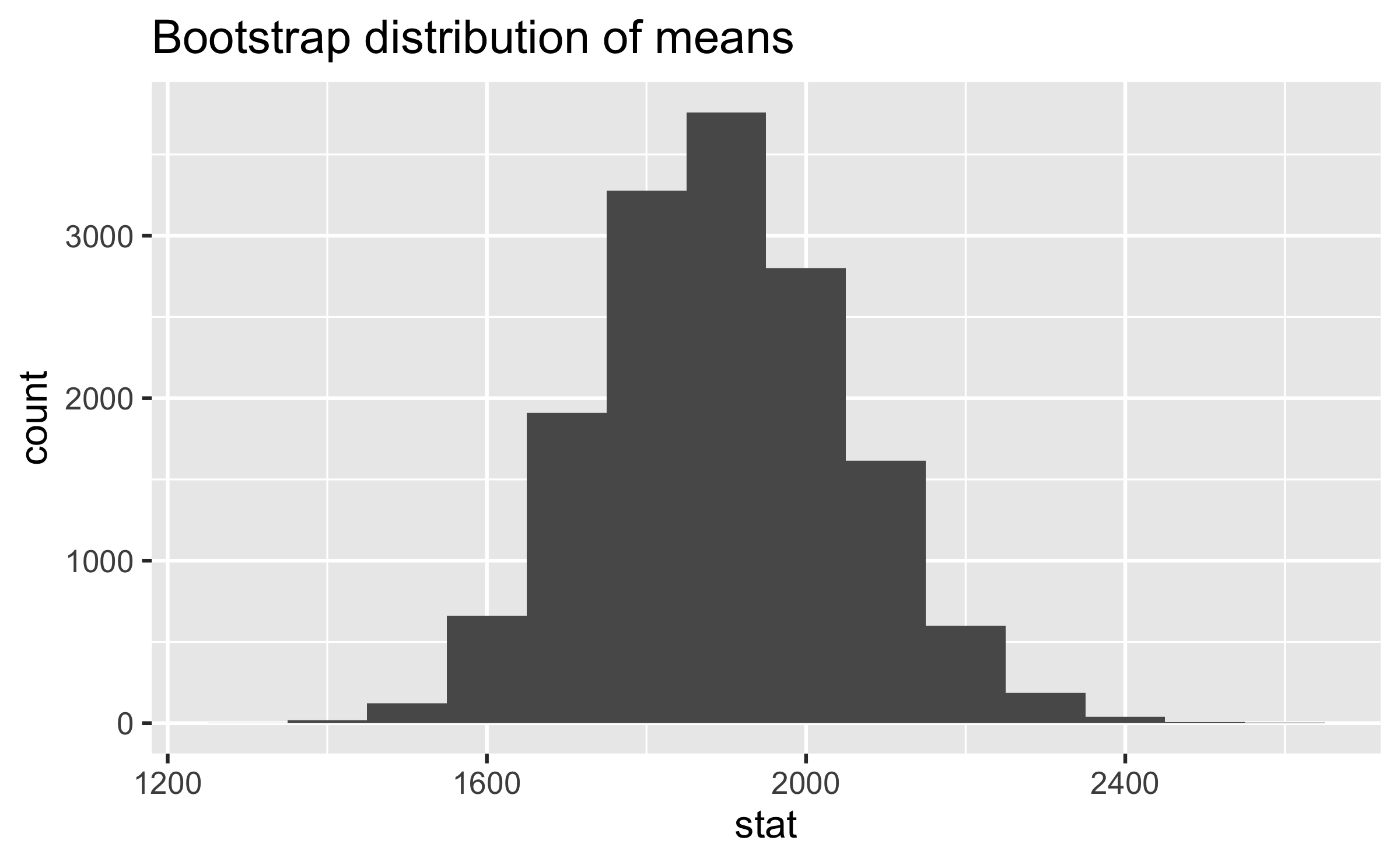
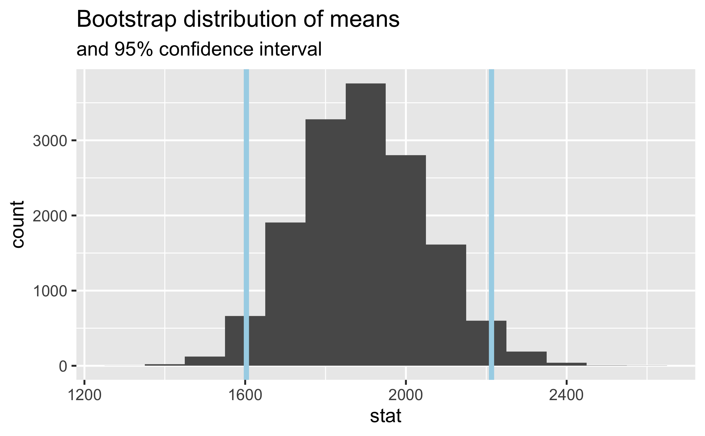
Visualize the confidence interval

17 / 24

Interpret the confidence interval

The 95% confidence interval for the mean rent of three bedroom flats in Edinburgh was calculated as (1603, 2213). Which of the following is the correct interpretation of this interval?

(a) 95% of the time the mean rent of three bedroom flats in this sample is between £1603 and £2213.

(b) 95% of all three bedroom flats in Edinburgh have rents between £1603 and £2213.

(c) We are 95% confident that the mean rent of all three bedroom flats is between £1603 and £2213.

(d) We are 95% confident that the mean rent of three bedroom flats in this sample is between £1603 and £2213.

18 / 24

Accuracy vs. precision

19 / 24

Confidence level

We are 95% confident that ...

  • Suppose we took many samples from the original population and built a 95% confidence interval based on each sample.
  • Then about 95% of those intervals would contain the true population parameter.
20 / 24

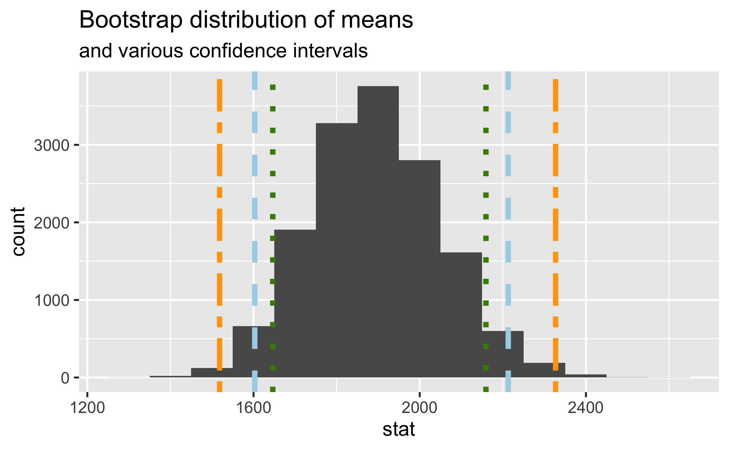
Commonly used confidence levels

Which line (orange dash/dot, blue dash, green dot) represents which confidence level?

21 / 24

Precision vs. accuracy

If we want to be very certain that we capture the population parameter, should we use a wider or a narrower interval? What drawbacks are associated with using a wider interval?

22 / 24

Precision vs. accuracy

If we want to be very certain that we capture the population parameter, should we use a wider or a narrower interval? What drawbacks are associated with using a wider interval?

22 / 24

Precision vs. accuracy

If we want to be very certain that we capture the population parameter, should we use a wider or a narrower interval? What drawbacks are associated with using a wider interval?

How can we get best of both worlds -- high precision and high accuracy?

22 / 24

Changing confidence level

How would you modify the following code to calculate a 90% confidence interval? How would you modify it for a 99% confidence interval?

edi_3br %>%
specify(response = rent) %>%
generate(reps = 15000, type = "bootstrap") %>%
calculate(stat = "mean") %>%
summarize(lower = quantile(stat, 0.025),
upper = quantile(stat, 0.975))
23 / 24

Recap

  • Sample statistic population parameter, but if the sample is good, it can be a good estimate
  • We report the estimate with a confidence interval, and the width of this interval depends on the variability of sample statistics from different samples from the population
  • Since we can't continue sampling from the population, we bootstrap from the one sample we have to estimate sampling variability
  • We can do this for any sample statistic:
    • For a mean: calculate(stat = "mean")
    • For a median: calculate(stat = "median")
    • Learn about calculating bootstrap intervals for other statistics in your homework
24 / 24

Rent in Edinburgh

2 / 24
Paused

Help

Keyboard shortcuts

, , Pg Up, k Go to previous slide
, , Pg Dn, Space, j Go to next slide
Home Go to first slide
End Go to last slide
Number + Return Go to specific slide
b / m / f Toggle blackout / mirrored / fullscreen mode
c Clone slideshow
p Toggle presenter mode
t Restart the presentation timer
?, h Toggle this help
Esc Back to slideshow