Inference overview

.title[
# Inference overview
]
.subtitle[
## <br><br> Data Science in a Box
]
.author[
### <a href="https://datasciencebox.org/">datasciencebox.org</a>
]

---

layout: true
  
<div class="my-footer">
<span>
<a href="https://datasciencebox.org" target="_blank">datasciencebox.org</a>
</span>
</div>

---

# Inference overview

---

## What do you want to do?

- Estimation -> Confidence interval
- Decision -> Hypothesis test
- First step: Ask the following questions
  - How many variables?
  - What types of variables?
  - What is the research question?

---

# Confidence intervals

---

## Confidence intervals

- Bootstrap
- Bounds: cutoff values for the middle XX% of the distribution
- Interpretation: We are XX% confident that the true population parameter is in the interval.
- Definition of confidence level: XX% of random samples of size n are expected to produce confidence intervals that contain the true population parameter.
- `infer::generate(reps, type = "bootstrap")`

---

## Confidence intervals exercises

- Note any assumptions you make in terms of sample size, observed sample statistic, etc.
- Imagine using index cards or chips to represent the data. 
- Specify whether the simulation type would be bootstrap, simulate, or permute.

]

---

## Accuracy vs. precision

.question[
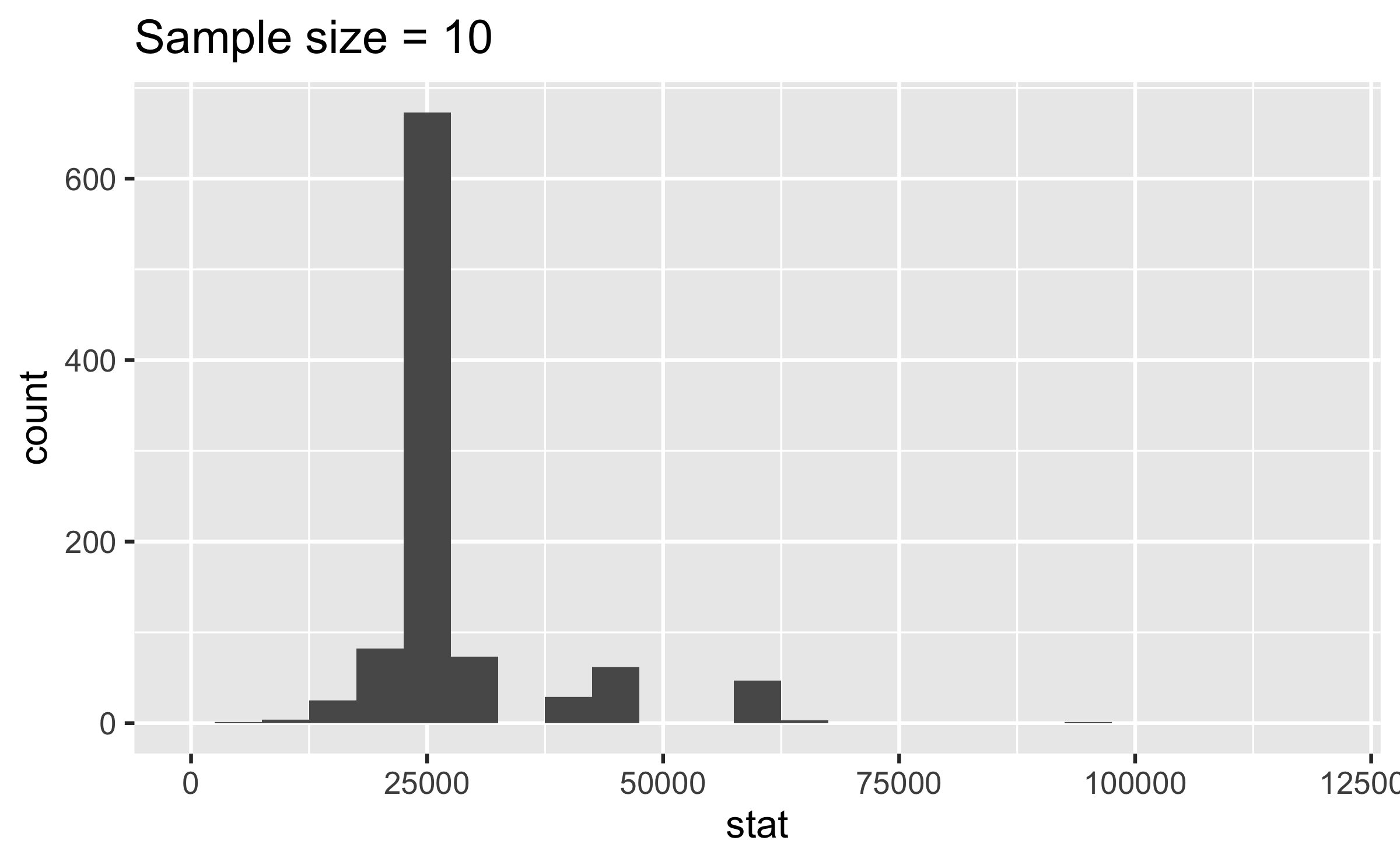
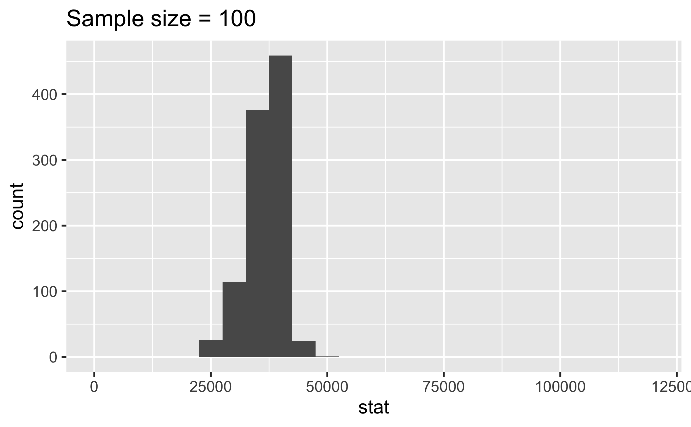
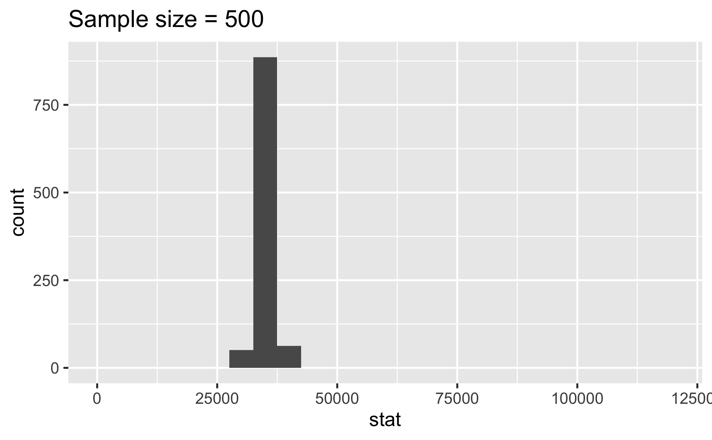
What happens to the width of the confidence interval as the confidence level increases? Why? Should we always prefer a confidence interval with a higher confidence level?
]

---

## Sample size and width of intervals

---

## Sample size and width of intervals

---

## Sample size and width of intervals

---

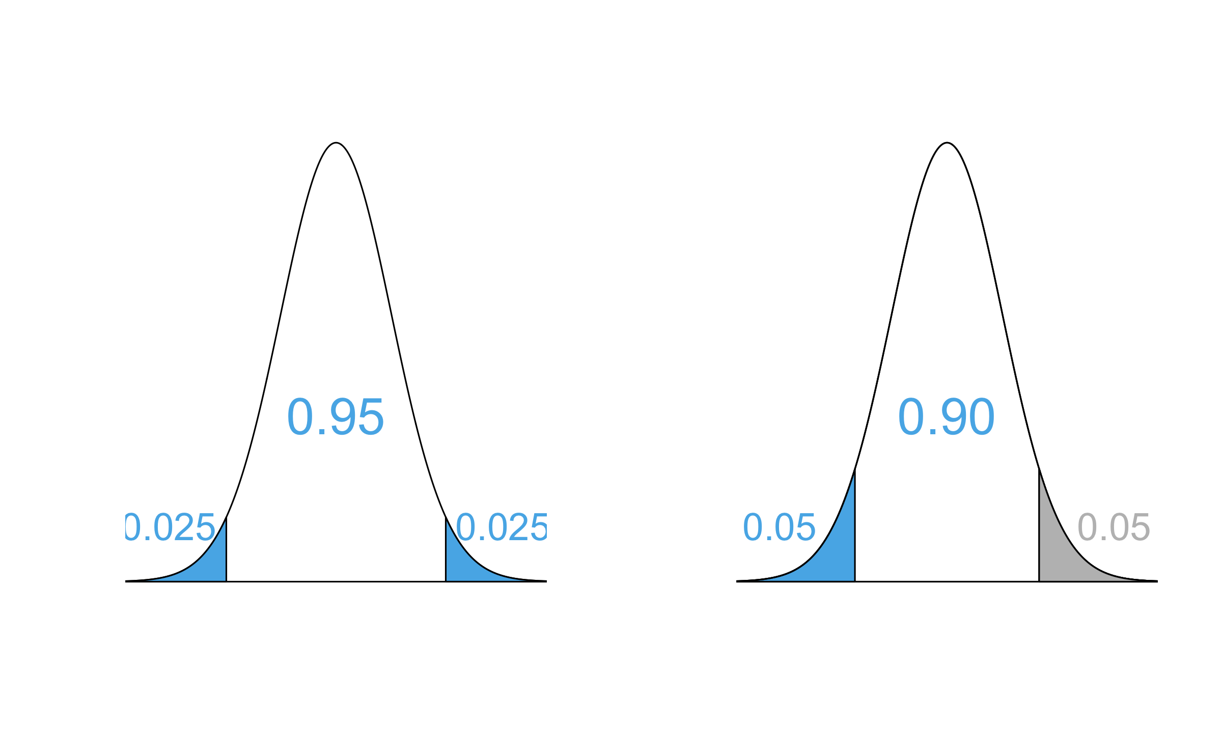
## Equivalency of confidence and significance levels

- Two sided alternative HT with `$\alpha$` `$\rightarrow$` `$CL = 1 - \alpha$`
- One sided alternative HT with `$\alpha$` `$\rightarrow$` `$CL = 1 - (2 \times \alpha)$`

---

## Interpretation of confidence intervals

<ul>
<li> The difference in price of a gallon of milk between Whole Foods and Harris Teeter is 30 cents.
<li> A gallon of milk costs 30 cents more at Whole Foods compared to Harris Teeter.
</ul>
</div>
]

.question[
What does your answer tell you about interpretation of confidence intervals for differences between two population parameters?
]

---

# Hypothesis tests

---

## Hypothesis testing

- Set the hypotheses.
- Calculate the observed sample statistic.
- Calculate the p-value.
- Make a conclusion, about the hypotheses, in context of the data and the research question.
- `infer::hypothesize(null = "point")` and `infer::generate(reps, type = "simulate")` or `infer::generate(reps, type = "bootstrap")`
- `infer::hypothesize(null = "independence")` and `infer::generate(reps, type = "permute")`
  
---

## Hypothesis testing exercises

- Note any assumptions you make in terms of sample size, observed sample statistic, etc.
- Imagine using index cards or chips to represent the data. 
- Specify whether the null hypothesis would be independence or point.
- Specify whether the simulation type would be bootstrap, simulate, or permute.
]

---

## Testing errors

- Type 1: Reject `$H_0$` when you shouldn't have
    - P(Type 1 error) = `$\alpha$`
- Type 2: Fail to reject `$H_0$` when you should have
    - P(Type 2 error) is harder to calculate, but increases as `$\alpha$` decreases

- Null hypothesis: Defendant is innocent
- Alternative hypothesis: Defendant is guilty

Which is worse: Type 1 or Type 2 error?
]

---

## Probabilities of testing errors

- P(Type 1 error) = `$\alpha$`
- P(Type 2 error) = 1 - Power
- Power = P(correctly rejecting the null hypothesis)

.question[
Fill in the blanks in terms of correctly/incorrectly rejecting/failing to reject the null hypothesis:

- `$\alpha$` is the probability of ______.
- 1 - Power is the probability of ______.
]

---

# Examples

---

## What do you want to do?

- Estimation -> Confidence interval
- Decision -> Hypothesis test
- First step: Ask the following questions
  - How many variables?
  - What type(s) of variable(s)?
  - What is the research question?

---

## Data: NC births

The dataset is in the `openintro` package.

```r
glimpse(ncbirths)
```

```
## Rows: 1,000
## Columns: 13
## $ fage           <int> NA, NA, 19, 21, NA, NA, 18, 17, NA, 20, …
## $ mage           <int> 13, 14, 15, 15, 15, 15, 15, 15, 16, 16, …
## $ mature         <fct> younger mom, younger mom, younger mom, y…
## $ weeks          <int> 39, 42, 37, 41, 39, 38, 37, 35, 38, 37, …
## $ premie         <fct> full term, full term, full term, full te…
## $ visits         <int> 10, 15, 11, 6, 9, 19, 12, 5, 9, 13, 9, 8…
## $ marital        <fct> not married, not married, not married, n…
## $ gained         <int> 38, 20, 38, 34, 27, 22, 76, 15, NA, 52, …
## $ weight         <dbl> 7.63, 7.88, 6.63, 8.00, 6.38, 5.38, 8.44…
## $ lowbirthweight <fct> not low, not low, not low, not low, not …
## $ gender         <fct> male, male, female, male, female, male, …
## $ habit          <fct> nonsmoker, nonsmoker, nonsmoker, nonsmok…
## $ whitemom       <fct> not white, not white, white, white, not …
```

---

## Length of gestation

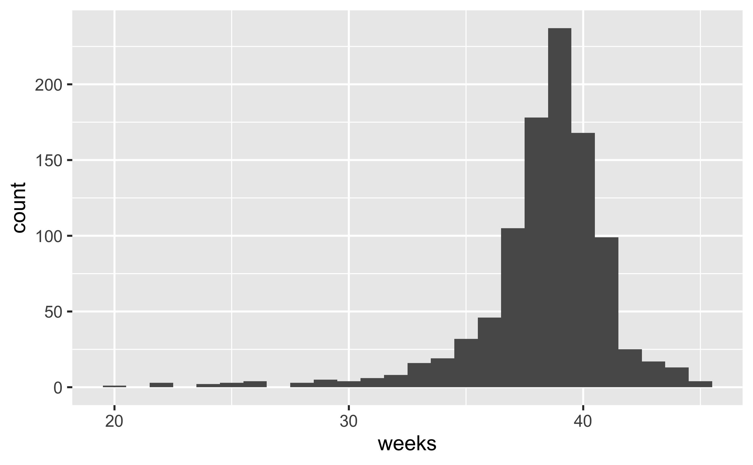
```
## # A tibble: 1 × 7
##     min  xbar   med     s    q1    q3   max
##   <int> <dbl> <dbl> <dbl> <dbl> <dbl> <int>
## 1    20  38.3    39  2.93    37    40    45
```

---

## Length of gestation

.question[
Assuming that this sample is representative of all births in NC, we are 95% confident that the average length of gestation for babies in NC is between ---- and ---- weeks.
]

**(1) How many variables?**

1 variable: length of gestation, `weeks`

**(2) What type(s) of variable(s)?**

Numerical

**(3) What is the research question?**

Estimate the average length of gestation `$\rightarrow$` confidence interval

---

## Simulation for CI for a mean

**Goal:** Use bootstrapping to estimate the sampling variability of the mean, i.e. the variability of means taken from the same population with the same sample size.

1. Take a bootstrap sample - a random sample taken with replacement from the 
original sample, of the same size as the original sample.

2. Calculate the mean of the bootstrap sample.

3. Repeat steps (1) and (2) many times to create a bootstrap distribution - 
a distribution of bootstrap means.

4. Calculate the bounds of the 95% confidence interval as the middle 95% 
of the bootstrap distribution.

---

## Set a seed first

From the documentation of `set.seed`:

- `set.seed` uses a single integer argument to set as many seeds as are required. There is no guarantee that different values of seed will seed the RNG differently, although any exceptions would be extremely rare.
- Initially, there is no seed; a new one is created from the current time and the process ID when one is required. Hence different sessions will give different simulation results, by default.

```r
set.seed(20180326)
```

---

## Computation for CI for a mean

```r
boot_means <- ncbirths %>%
  filter(!is.na(weeks)) %>% # remove NAs
  specify(response = weeks) %>%
  generate(reps = 1000, type = "bootstrap") %>%
  calculate(stat = "mean")
ggplot(data = boot_means, aes(x = stat)) +
  geom_histogram(binwidth = 0.03)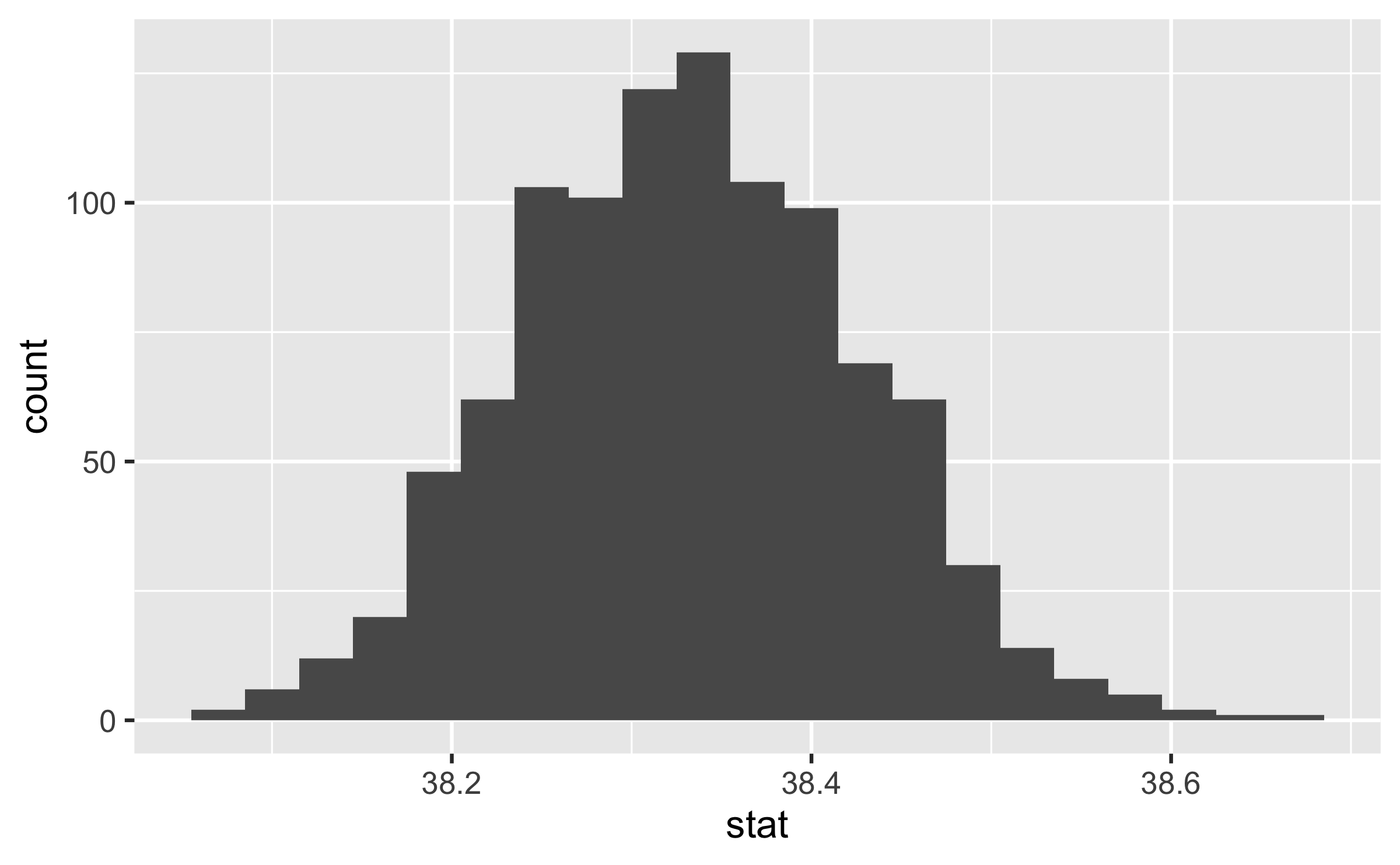
```

---

## Length of gestation

```r
boot_means %>%
  summarise(
    lower = quantile(stat, 0.025),
    upper = quantile(stat, 0.975)
  )
```

```
## # A tibble: 1 × 2
##   lower upper
##   <dbl> <dbl>
## 1  38.2  38.5
```

Assuming that this sample is representative of all births in NC, we are 95% confident that the average length of gestation for babies in NC is between 38.1 and 38.5 weeks.

---

## Length of gestation, revisited

.question[
The average length of human gestation is 280 days, or 40 weeks, from the first day of the woman's last menstrual period. Do these data provide convincing evidence that average length of gestation for women in NC is different than 40 weeks? Use a significance level of 5%.
]

`$H_0: \mu = 40$`  
`$H_A: \mu \ne 40$`

- We just said, "we are 95% confident that the average length of gestation for babies in NC is between 38.1 and 38.5 weeks".

- Since the null value is outside the CI, we would reject the null hypothesis in favor of the alternative.

- But an alternative, more direct, way of answering this question is using a hypothesis test.

---

## Simulation for HT for a mean

**Goal:** Use bootstrapping to generate a sampling distribution under the assumption of the null hypothesis being true. Then, calculate the p-value to make a decision on the hypotheses.

1. Take a bootstrap sample - a random sample taken with replacement from the 
original sample, of the same size as the original sample.

2. Calculate the mean of the bootstrap sample.

3. Repeat steps (1) and (2) many times to create a bootstrap distribution - 
a distribution of bootstrap means.

4. Shift the bootstrap distribution to be centered at the null value by subtracting/adding the difference between the center of the bootstrap distribution and the null value to each bootstrap mean.

5. Calculate the p-value as the proportion of simulations that yield a sample mean at least as extreme as the observed sample mean.

---

## Computation for HT for a mean

```r
boot_means_shifted <- ncbirths %>%
  filter(!is.na(weeks)) %>% # remove NAs
  specify(response = weeks) %>%
  hypothesize(null = "point", mu = 40) %>% # hypothesize step
  generate(reps = 1000, type = "bootstrap") %>%
  calculate(stat = "mean")
ggplot(data = boot_means_shifted, aes(x = stat)) +
  geom_histogram(binwidth = 0.03) +
  geom_vline(xintercept = 38.33, color = "red") +
  geom_vline(xintercept = 40 + (40 - 38.33), color = "red")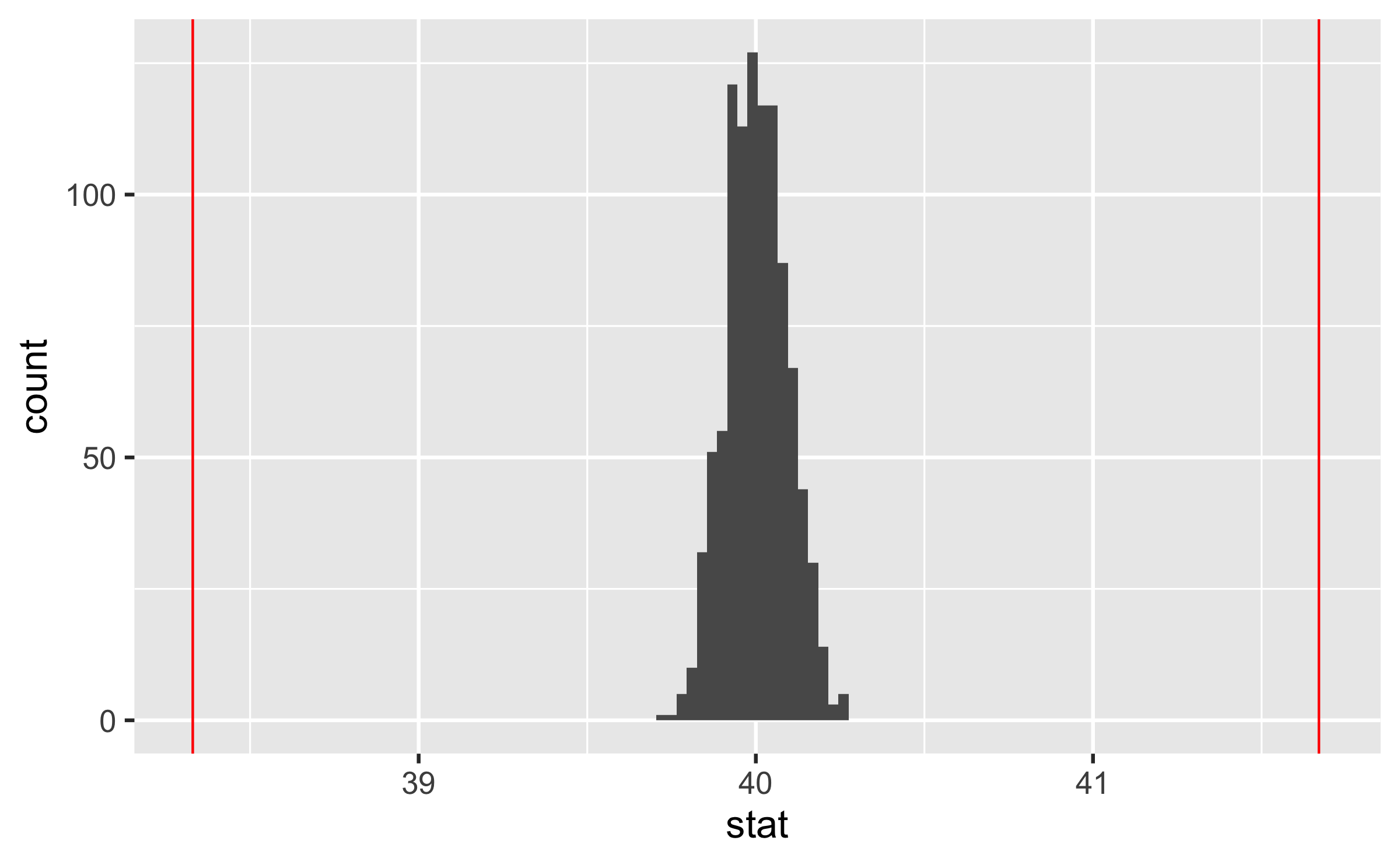
```

---

## Length of gestation

```r
boot_means_shifted %>%
  filter(stat <= 38.33) %>%
  summarise(p_value = 2 * (n() / 1000))
```

```
## # A tibble: 1 × 1
##   p_value
##     <dbl>
## 1       0
```

Since p-value less than the significance level, we reject the null hypothesis. The data provide convincing evidence that the average length of gestation of births in NC is different than 40.

---

## **infer** structure

```r
df %>%
  specify(response, explanatory) %>% # explanatory optional
  generate(reps, type) %>% # type: bootstrap, simulate, or permute
  calculate(stat)
```

- Always start with data frame
- Result is always a data frame with a variable called `stat`
   - See the documentation for `calculate` to see which `stat`istics can be calculated
- For hypothesis testing add a `hypothesize()` step between `specify()` and `generate()`
    - `null = "point"`, and then specify the null value
    - `null = "independence"`