Recoding data

Data Science in a Box

datasciencebox.org

1 / 19

Case study: Religion and income

2 / 19

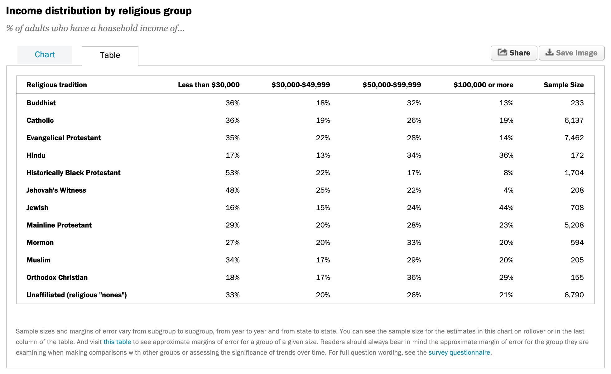
Source: pewforum.org/religious-landscape-study/income-distribution, Retrieved 14 April, 2020

3 / 19

Read data

library(readxl)
rel_inc <- read_excel("data/relig-income.xlsx")

## # A tibble: 12 × 6
##   `Religious tradition`         `Less than $30…` `$30,000-$49,9…`
##   <chr>                                    <dbl>            <dbl>
## 1 Buddhist                                  0.36             0.18
## 2 Catholic                                  0.36             0.19
## 3 Evangelical Protestant                    0.35             0.22
## 4 Hindu                                     0.17             0.13
## 5 Historically Black Protestant             0.53             0.22
## 6 Jehovah's Witness                         0.48             0.25
## # … with 6 more rows, and 3 more variables:
## #   `$50,000-$99,999` <dbl>, `$100,000 or more` <dbl>,
## #   `Sample Size` <dbl>

4 / 19

Rename columns

rel_inc %>%
  rename( 
    religion = `Religious tradition`, 
    n = `Sample Size` 
  )

## # A tibble: 12 × 6
##   religion     `Less than $30…` `$30,000-$49,9…` `$50,000-$99,9…`
##   <chr>                   <dbl>            <dbl>            <dbl>
## 1 Buddhist                 0.36             0.18             0.32
## 2 Catholic                 0.36             0.19             0.26
## 3 Evangelical…             0.35             0.22             0.28
## 4 Hindu                    0.17             0.13             0.34
## 5 Historicall…             0.53             0.22             0.17
## 6 Jehovah's W…             0.48             0.25             0.22
## # … with 6 more rows, and 2 more variables:
## #   `$100,000 or more` <dbl>, n <dbl>

5 / 19

If we want a new variable called income with levels such as "Less than $30,000", "$30,000-$49,999", ... etc. which function should we use?

## # A tibble: 48 × 4
##    religion                   n income            proportion
##    <chr>                  <dbl> <chr>                  <dbl>
##  1 Buddhist                 233 Less than $30,000       0.36
##  2 Buddhist                 233 $30,000-$49,999         0.18
##  3 Buddhist                 233 $50,000-$99,999         0.32
##  4 Buddhist                 233 $100,000 or more        0.13
##  5 Catholic                6137 Less than $30,000       0.36
##  6 Catholic                6137 $30,000-$49,999         0.19
##  7 Catholic                6137 $50,000-$99,999         0.26
##  8 Catholic                6137 $100,000 or more        0.19
##  9 Evangelical Protestant  7462 Less than $30,000       0.35
## 10 Evangelical Protestant  7462 $30,000-$49,999         0.22
## 11 Evangelical Protestant  7462 $50,000-$99,999         0.28
## 12 Evangelical Protestant  7462 $100,000 or more        0.14
## 13 Hindu                    172 Less than $30,000       0.17
## 14 Hindu                    172 $30,000-$49,999         0.13
## 15 Hindu                    172 $50,000-$99,999         0.34
## # … with 33 more rows

6 / 19

datasciencebox.org

Pivot longerrel_inc %>%
  rename(
    religion = `Religious tradition`,
    n = `Sample Size`
  ) %>%
  pivot_longer( 
    cols = -c(religion, n),   # all but religion and n 
    names_to = "income",  
    values_to = "proportion" 
  )

## # A tibble: 48 × 4
##   religion     n income            proportion
##   <chr>    <dbl> <chr>                  <dbl>
## 1 Buddhist   233 Less than $30,000       0.36
## 2 Buddhist   233 $30,000-$49,999         0.18
## 3 Buddhist   233 $50,000-$99,999         0.32
## 4 Buddhist   233 $100,000 or more        0.13
## 5 Catholic  6137 Less than $30,000       0.36
## 6 Catholic  6137 $30,000-$49,999         0.19
## # … with 42 more rows
7 / 19

Calculate frequencies

rel_inc %>%
  rename(
    religion = `Religious tradition`,
    n = `Sample Size`
  ) %>%
  pivot_longer(
    cols = -c(religion, n), 
    names_to = "income", 
    values_to = "proportion"
  ) %>%
  mutate(frequency = round(proportion * n))

## # A tibble: 48 × 5
##   religion     n income            proportion frequency
##   <chr>    <dbl> <chr>                  <dbl>     <dbl>
## 1 Buddhist   233 Less than $30,000       0.36        84
## 2 Buddhist   233 $30,000-$49,999         0.18        42
## 3 Buddhist   233 $50,000-$99,999         0.32        75
## 4 Buddhist   233 $100,000 or more        0.13        30
## 5 Catholic  6137 Less than $30,000       0.36      2209
## 6 Catholic  6137 $30,000-$49,999         0.19      1166
## # … with 42 more rows

8 / 19

Save data

rel_inc_long <- rel_inc %>% 
  rename(
    religion = `Religious tradition`,
    n = `Sample Size`
  ) %>%
  pivot_longer(
    cols = -c(religion, n), 
    names_to = "income", 
    values_to = "proportion"
  ) %>%
  mutate(frequency = round(proportion * n))

9 / 19

Barplot

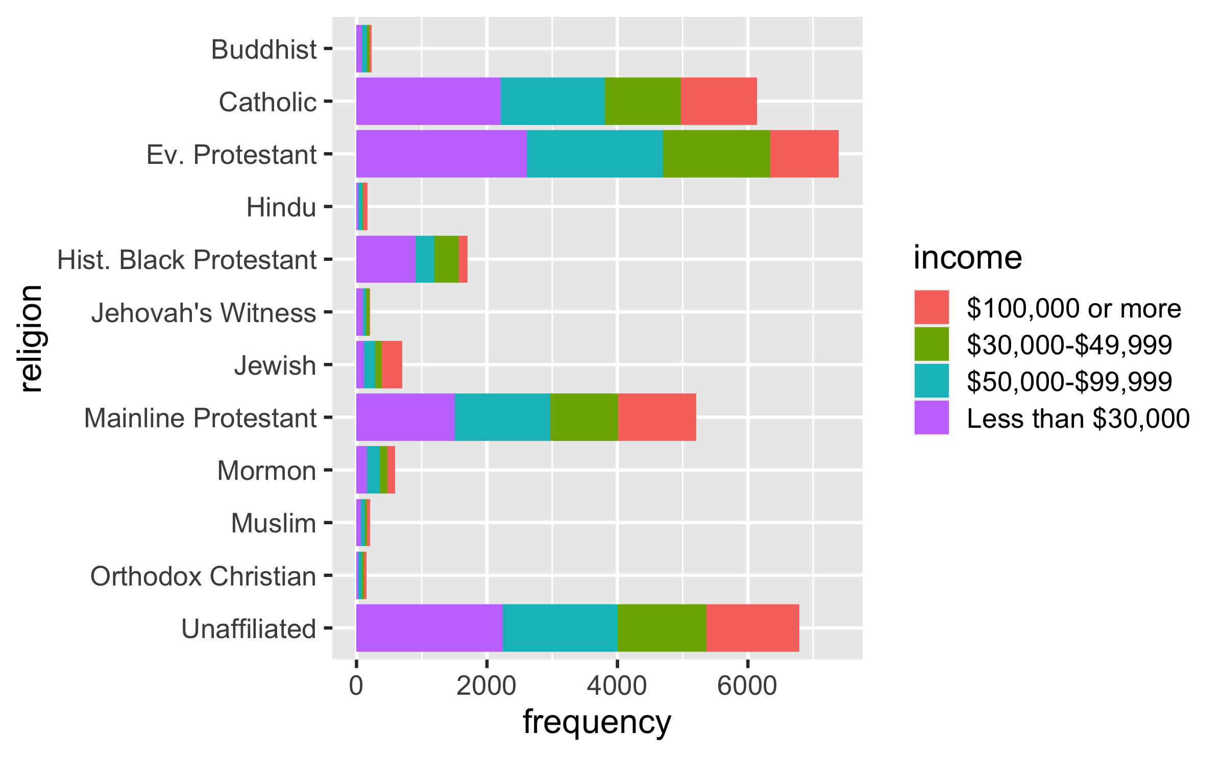
ggplot(rel_inc_long, aes(y = religion, x = frequency)) +
  geom_col()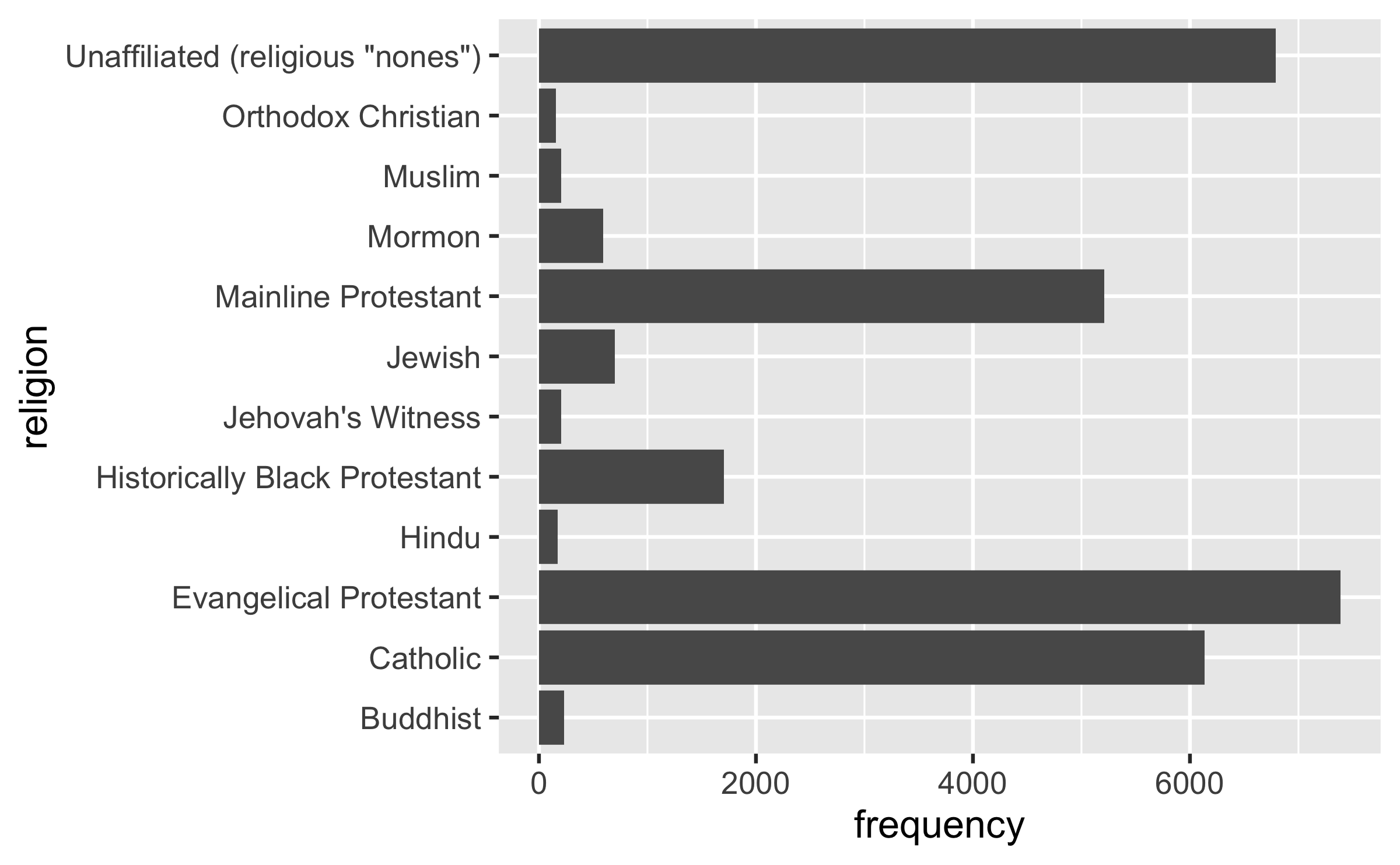

10 / 19

Recode religion

rel_inc_long <- rel_inc_long %>%
  mutate(religion = case_when(
    religion == "Evangelical Protestant"           ~ "Ev. Protestant",
    religion == "Historically Black Protestant"    ~ "Hist. Black Protestant",
    religion == 'Unaffiliated (religious "nones")' ~ "Unaffiliated",
    TRUE                                           ~ religion
  ))

11 / 19

Reverse religion order

rel_inc_long <- rel_inc_long %>%
  mutate(religion = fct_rev(religion))

12 / 19

Add income

ggplot(rel_inc_long, aes(y = religion, x = frequency, fill = income)) + 
  geom_col()

13 / 19

Fill bars

ggplot(rel_inc_long, aes(y = religion, x = frequency, fill = income)) +
  geom_col(position = "fill")

14 / 19

Change colors

ggplot(rel_inc_long, aes(y = religion, x = frequency, fill = income)) +
  geom_col(position = "fill") +
  scale_fill_viridis_d()

15 / 19

Change theme

ggplot(rel_inc_long, aes(y = religion, x = frequency, fill = income)) +
  geom_col(position = "fill") +
  scale_fill_viridis_d() +
  theme_minimal()

16 / 19

Move legend to the bottom

ggplot(rel_inc_long, aes(y = religion, x = frequency, fill = income)) +
  geom_col(position = "fill") +
  scale_fill_viridis_d() +
  theme_minimal() +
  theme(legend.position = "bottom")

17 / 19

Legend adjustments

ggplot(rel_inc_long, aes(y = religion, x = frequency, fill = income)) +
  geom_col(position = "fill") +
  scale_fill_viridis_d() +
  theme_minimal() +
  theme(legend.position = "bottom") +
  guides(fill = guide_legend(nrow = 2, byrow = TRUE))

18 / 19

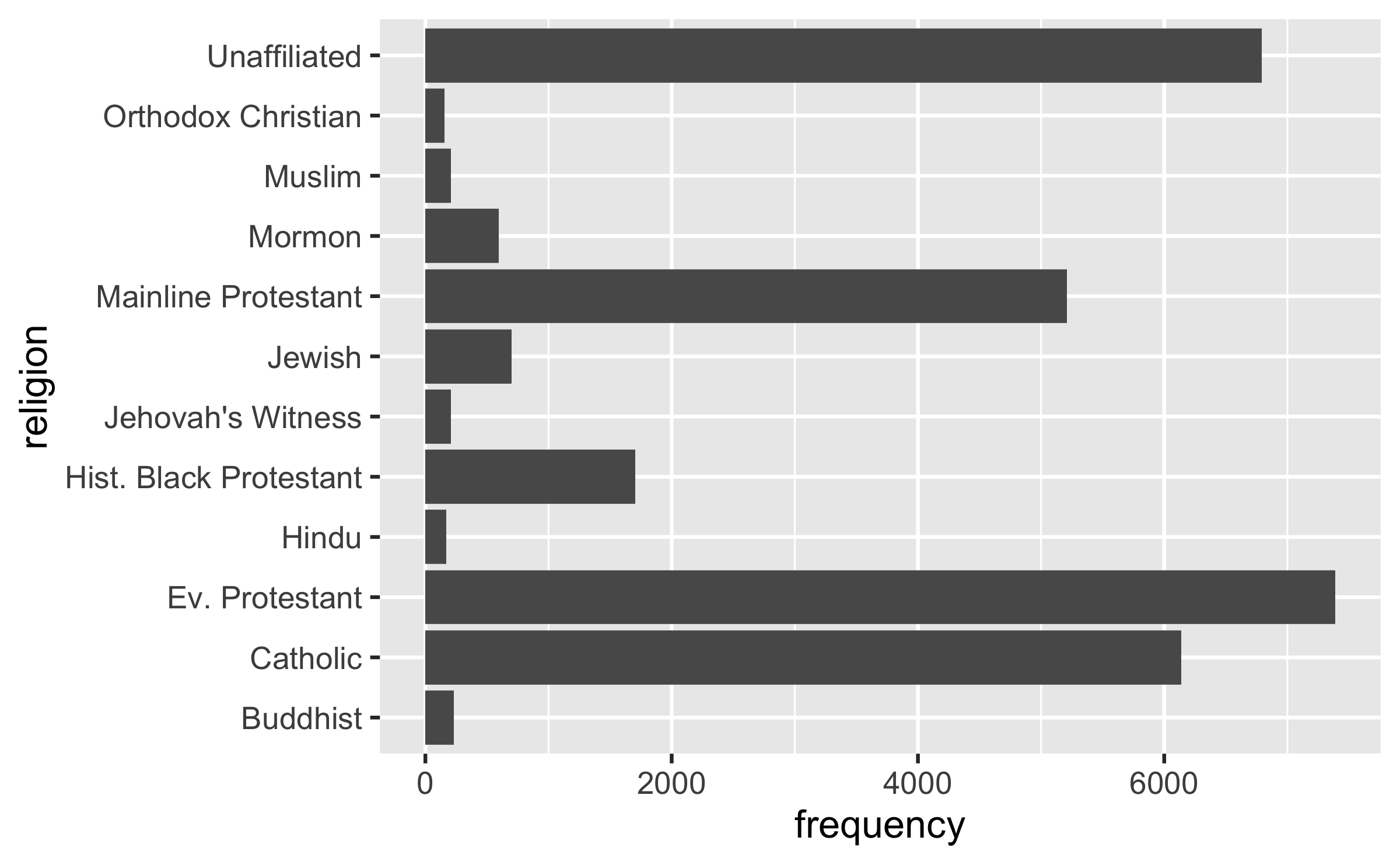
Fix labels

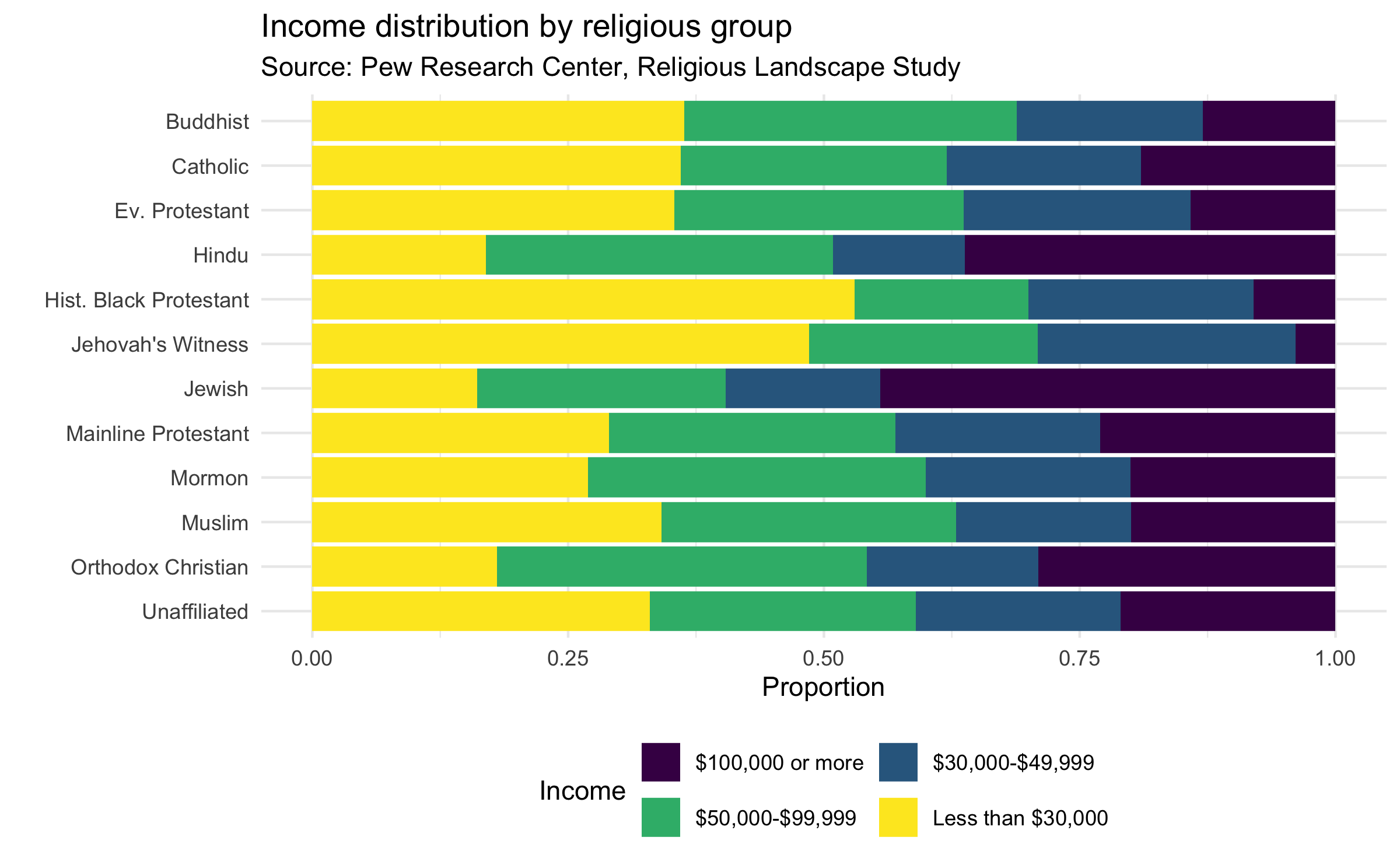
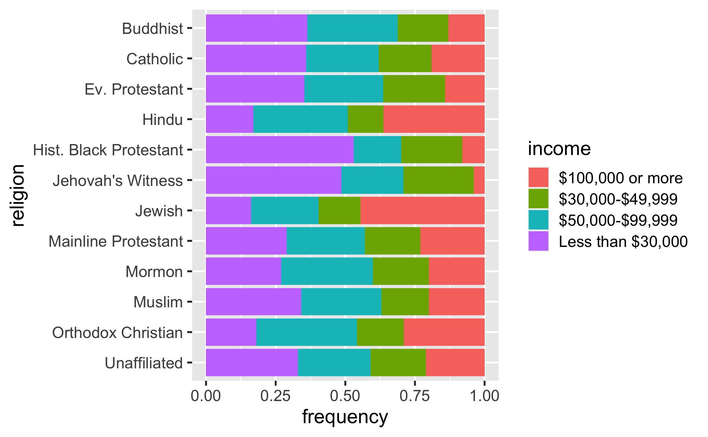
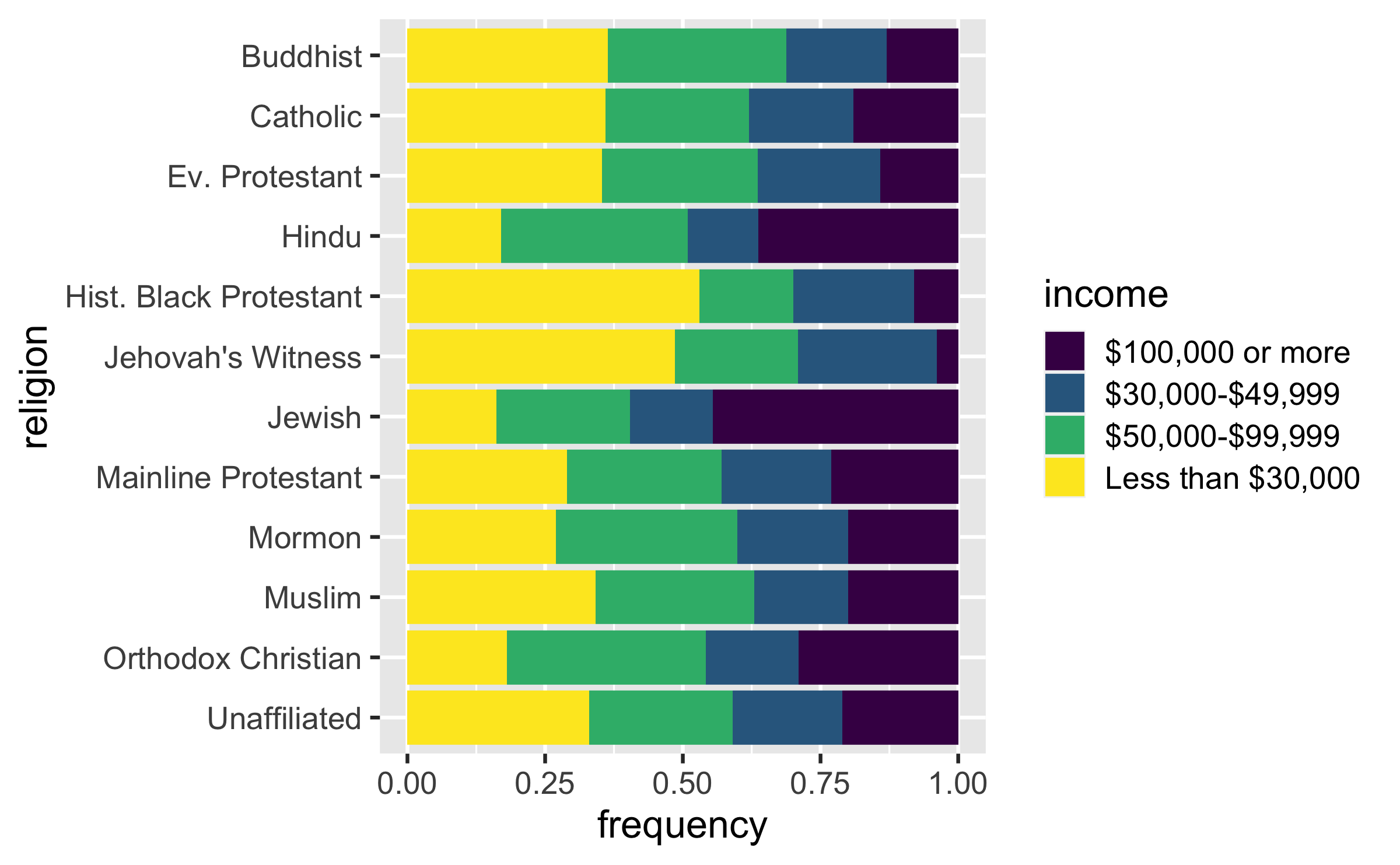
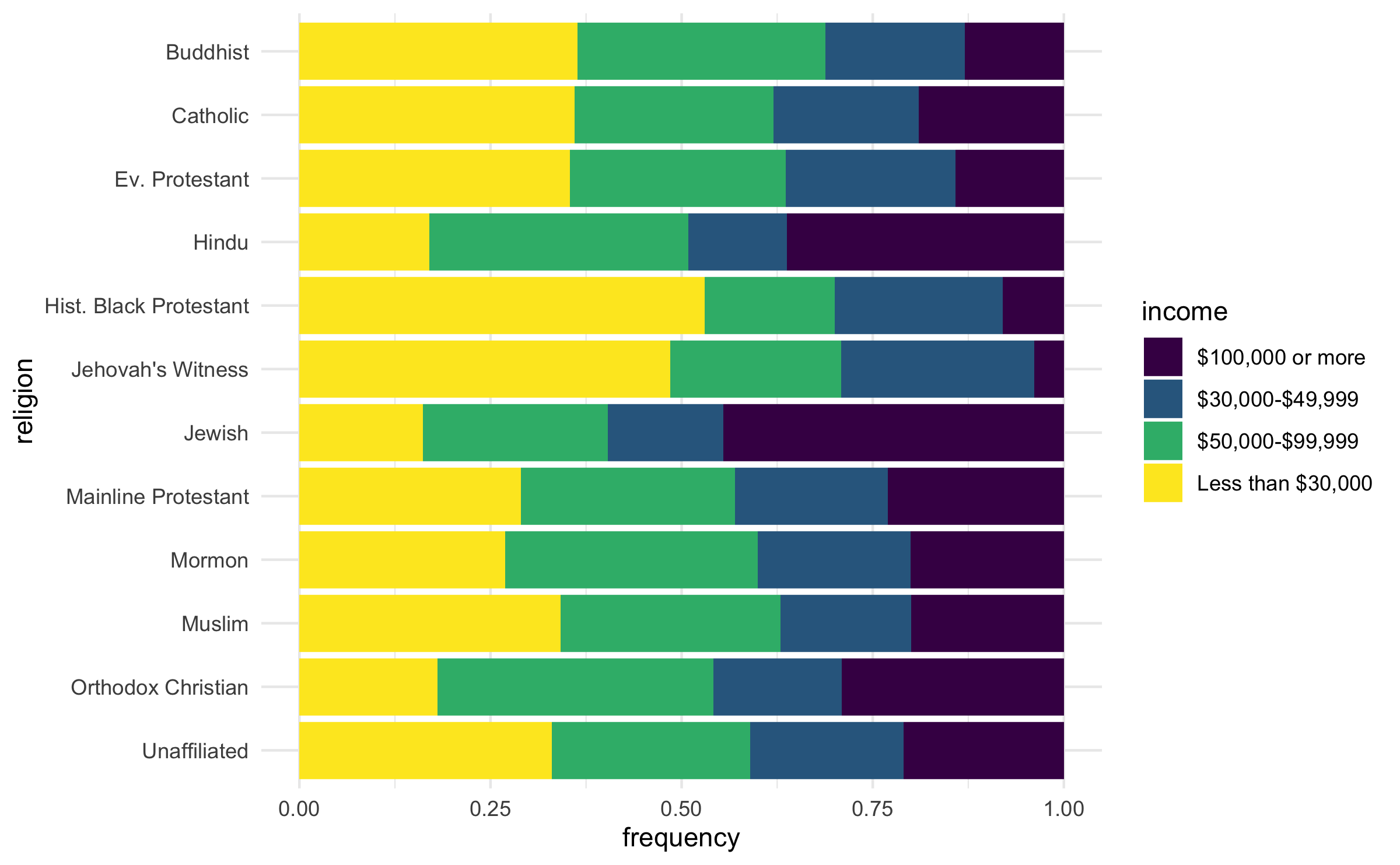
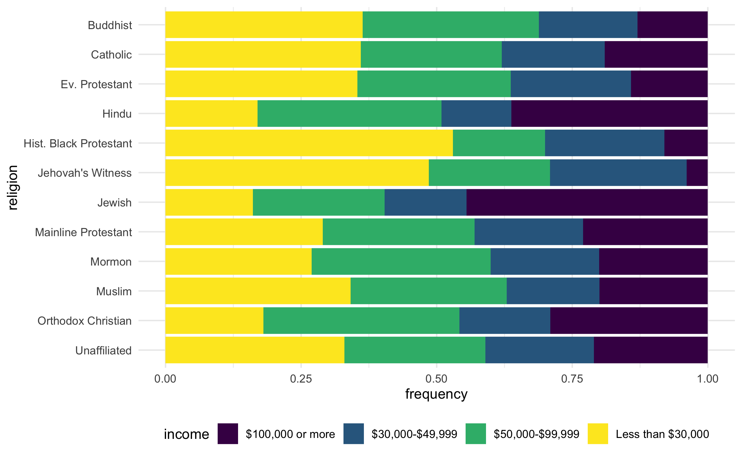
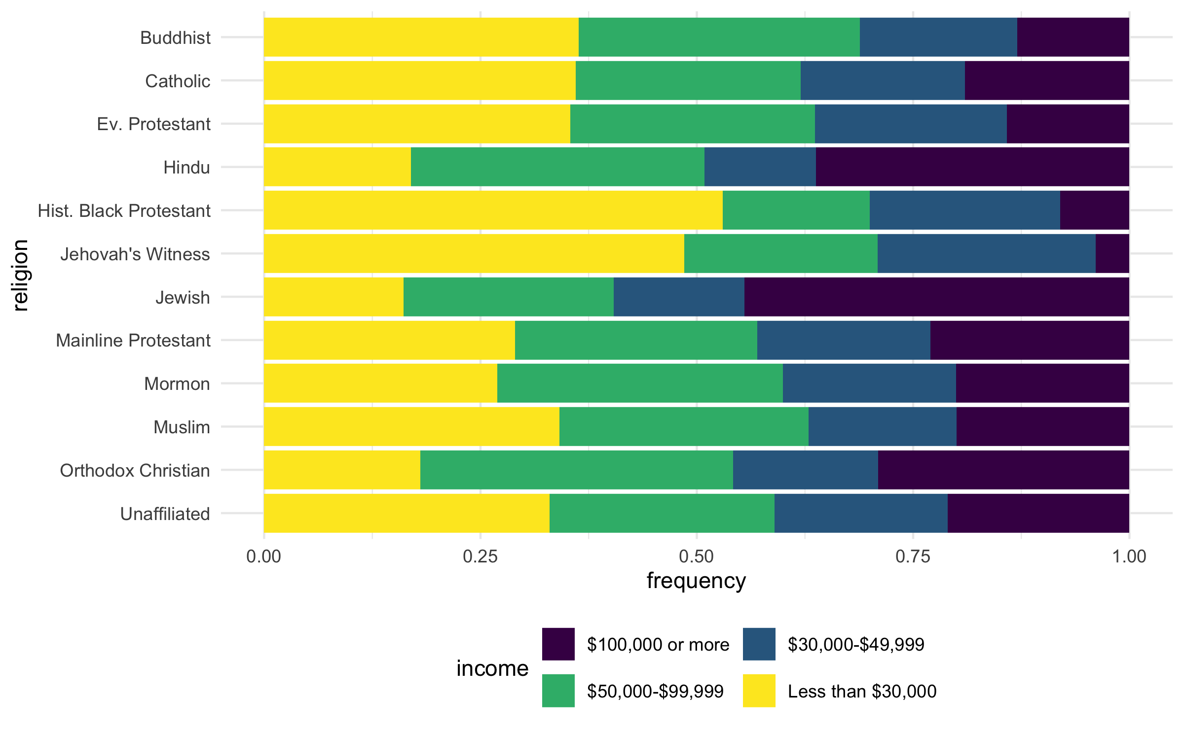
ggplot(rel_inc_long, aes(y = religion, x = frequency, fill = income)) +
  geom_col(position = "fill") +
  scale_fill_viridis_d() +
  theme_minimal() +
  theme(legend.position = "bottom") +
  guides(fill = guide_legend(nrow = 2, byrow = TRUE)) +
  labs(
    x = "Proportion", y = "", 
    title = "Income distribution by religious group", 
    subtitle = "Source: Pew Research Center, Religious Landscape Study", 
    fill = "Income" 
    )

↑, ←, Pg Up, k	Go to previous slide
↓, →, Pg Dn, Space, j	Go to next slide
Home	Go to first slide
End	Go to last slide
Number + Return	Go to specific slide
b / m / f	Toggle blackout / mirrored / fullscreen mode
c	Clone slideshow
p	Toggle presenter mode
t	Restart the presentation timer
?, h	Toggle this help

Recoding data

Data Science in a Box

datasciencebox.org

Case study: Religion and income

Read data

Rename columns

Pivot longer

Calculate frequencies

Save data

Barplot

Recode religion

Reverse religion order

Add income

Fill bars

Change colors

Change theme

Move legend to the bottom

Legend adjustments

Fix labels

Case study: Religion and income

Help