Five core activities of data analysis
- Stating and refining the question
- Exploring the data
- Building formal statistical models
- Interpreting the results
- Communicating the results
Roger D. Peng and Elizabeth Matsui. "The Art of Data Science." A Guide for Anyone Who Works with Data. Skybrude Consulting, LLC (2015).
Six types of questions
- Descriptive: summarize a characteristic of a set of data
- Exploratory: analyze to see if there are patterns, trends, or relationships between variables (hypothesis generating)
- Inferential: analyze patterns, trends, or relationships in representative data from a population
- Predictive: make predictions for individuals or groups of individuals
- Causal: whether changing one factor will change another factor, on average, in a population
- Mechanistic: explore "how" as opposed to whether
Jeffery T. Leek and Roger D. Peng. "What is the question?." Science 347.6228 (2015): 1314-1315.
Ex: COVID-19 and Vitamin D
- Descriptive: frequency of hospitalisations due to COVID-19 in a set of data collected from a group of individuals
Ex: COVID-19 and Vitamin D
- Descriptive: frequency of hospitalisations due to COVID-19 in a set of data collected from a group of individuals
- Exploratory: examine relationships between a range of dietary factors and COVID-19 hospitalisations
Ex: COVID-19 and Vitamin D
- Descriptive: frequency of hospitalisations due to COVID-19 in a set of data collected from a group of individuals
- Exploratory: examine relationships between a range of dietary factors and COVID-19 hospitalisations
- Inferential: examine whether any relationship between taking Vitamin D supplements and COVID-19 hospitalisations found in the sample hold for the population at large
- Predictive: what types of people will take Vitamin D supplements during the next year
- Causal: whether people with COVID-19 who were randomly assigned to take Vitamin D supplements or those who were not are hospitalised
- Mechanistic: how increased vitamin D intake leads to a reduction in the number of viral illnesses
Questions to data science problems
- Do you have appropriate data to answer your question?
- Do you have information on confounding variables?
- Was the data you're working with collected in a way that introduces bias?
Questions to data science problems
- Do you have appropriate data to answer your question?
- Do you have information on confounding variables?
- Was the data you're working with collected in a way that introduces bias?
Suppose I want to estimate the average number of children in households in Edinburgh. I conduct a survey at an elementary school in Edinburgh and ask students at this elementary school how many children, including themselves, live in their house. Then, I take the average of the responses. Is this a biased or an unbiased estimate of the number of children in households in Edinburgh? If biased, will the value be an overestimate or underestimate?
Checklist
- Formulate your question
- Read in your data
- Check the dimensions
- Look at the top and the bottom of your data
- Validate with at least one external data source
- Make a plot
- Try the easy solution first
Formulate your question
- Consider scope:
- Are air pollution levels higher on the east coast than on the west coast?
- Are hourly ozone levels on average higher in New York City than they are in Los Angeles?
- Do counties in the eastern United States have higher ozone levels than counties in the western United States?
- Most importantly: "Do I have the right data to answer this question?"
Read in your data
- Place your data in a folder called
data - Read it into R with
read_csv()or friends (read_delim(),read_excel(), etc.)
library(readxl)fav_food <- read_excel("data/favourite-food.xlsx")fav_food## # A tibble: 5 × 6## `Student ID` `Full Name` favourite.food mealPlan AGE SES ## <dbl> <chr> <chr> <chr> <chr> <chr>## 1 1 Sunil Huffmann Strawberry yo… Lunch o… 4 High ## 2 2 Barclay Lynn French fries Lunch o… 5 Midd…## 3 3 Jayendra Lyne N/A Breakfa… 7 Low ## 4 4 Leon Rossini Anchovies Lunch o… 99999 Midd…## 5 5 Chidiegwu Dun… Pizza Breakfa… five Highclean_names()
If the variable names are malformatted, use janitor::clean_names()
library(janitor)fav_food %>% clean_names()## # A tibble: 5 × 6## student_id full_name favourite_food meal_plan age ses ## <dbl> <chr> <chr> <chr> <chr> <chr>## 1 1 Sunil Huffmann Strawberry yo… Lunch on… 4 High ## 2 2 Barclay Lynn French fries Lunch on… 5 Midd…## 3 3 Jayendra Lyne N/A Breakfas… 7 Low ## 4 4 Leon Rossini Anchovies Lunch on… 99999 Midd…## 5 5 Chidiegwu Dunk… Pizza Breakfas… five HighCase study: NYC Squirrels!
- The Squirrel Census is a multimedia science, design, and storytelling project focusing on the Eastern gray (Sciurus carolinensis). They count squirrels and present their findings to the public.
- This table contains squirrel data for each of the 3,023 sightings, including location coordinates, age, primary and secondary fur color, elevation, activities, communications, and interactions between squirrels and with humans.
#install_github("mine-cetinkaya-rundel/nycsquirrels18")library(nycsquirrels18)Locate the codebook
mine-cetinkaya-rundel.github.io/nycsquirrels18/reference/squirrels.html
Check the dimensions
dim(squirrels)## [1] 3023 35Look at the top...
squirrels %>% head()## # A tibble: 6 × 35## long lat unique_squirrel_id hectare shift date ## <dbl> <dbl> <chr> <chr> <chr> <date> ## 1 -74.0 40.8 13A-PM-1014-04 13A PM 2018-10-14## 2 -74.0 40.8 15F-PM-1010-06 15F PM 2018-10-10## 3 -74.0 40.8 19C-PM-1018-02 19C PM 2018-10-18## 4 -74.0 40.8 21B-AM-1019-04 21B AM 2018-10-19## 5 -74.0 40.8 23A-AM-1018-02 23A AM 2018-10-18## 6 -74.0 40.8 38H-PM-1012-01 38H PM 2018-10-12## # … with 29 more variables: hectare_squirrel_number <dbl>,## # age <chr>, primary_fur_color <chr>,## # highlight_fur_color <chr>,## # combination_of_primary_and_highlight_color <chr>,## # color_notes <chr>, location <chr>,## # above_ground_sighter_measurement <chr>,## # specific_location <chr>, running <lgl>, chasing <lgl>, …...and the bottom
squirrels %>% tail()## # A tibble: 6 × 35## long lat unique_squirrel_id hectare shift date ## <dbl> <dbl> <chr> <chr> <chr> <date> ## 1 -74.0 40.8 6D-PM-1020-01 06D PM 2018-10-20## 2 -74.0 40.8 21H-PM-1018-01 21H PM 2018-10-18## 3 -74.0 40.8 31D-PM-1006-02 31D PM 2018-10-06## 4 -74.0 40.8 37B-AM-1018-04 37B AM 2018-10-18## 5 -74.0 40.8 21C-PM-1006-01 21C PM 2018-10-06## 6 -74.0 40.8 7G-PM-1018-04 07G PM 2018-10-18## # … with 29 more variables: hectare_squirrel_number <dbl>,## # age <chr>, primary_fur_color <chr>,## # highlight_fur_color <chr>,## # combination_of_primary_and_highlight_color <chr>,## # color_notes <chr>, location <chr>,## # above_ground_sighter_measurement <chr>,## # specific_location <chr>, running <lgl>, chasing <lgl>, …Validate with at least one external data source
## # A tibble: 3,023 × 2## long lat## <dbl> <dbl>## 1 -74.0 40.8## 2 -74.0 40.8## 3 -74.0 40.8## 4 -74.0 40.8## 5 -74.0 40.8## 6 -74.0 40.8## 7 -74.0 40.8## 8 -74.0 40.8## 9 -74.0 40.8## 10 -74.0 40.8## 11 -74.0 40.8## 12 -74.0 40.8## 13 -74.0 40.8## 14 -74.0 40.8## 15 -74.0 40.8## # … with 3,008 more rows
Make a plot
ggplot(squirrels, aes(x = long, y = lat)) + geom_point(alpha = 0.2)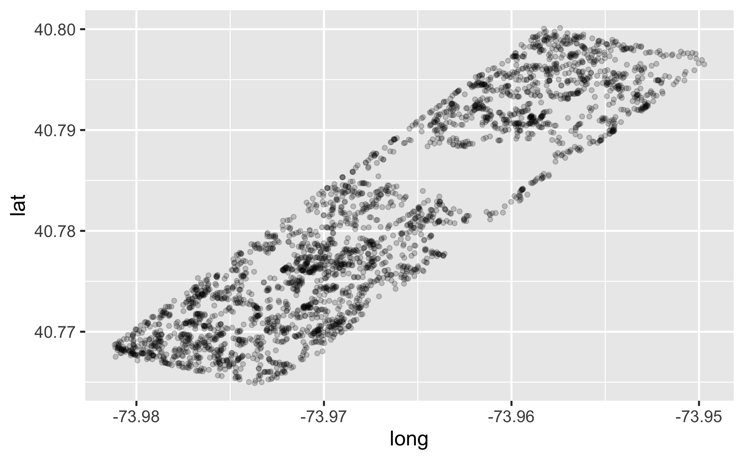
Make a plot
ggplot(squirrels, aes(x = long, y = lat)) + geom_point(alpha = 0.2)
Hypothesis: There will be a higher density of sightings on the perimeter than inside the park.
Try the easy solution first
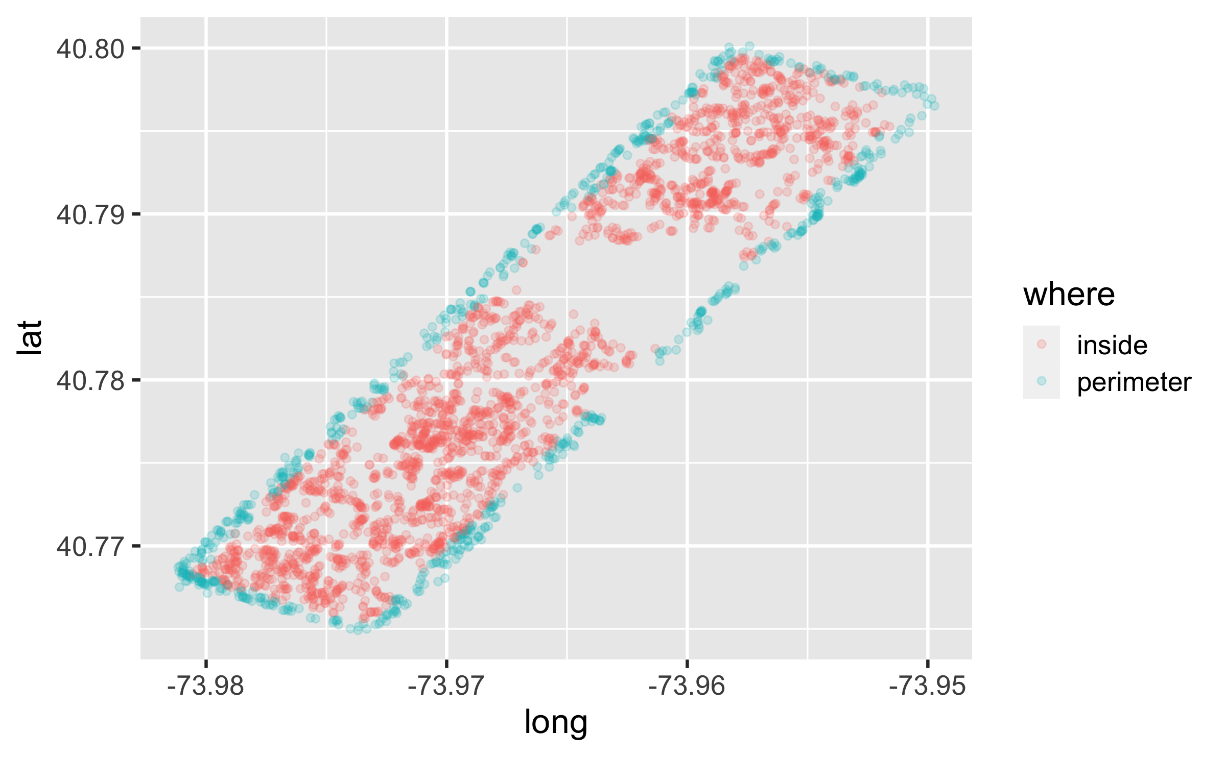
squirrels <- squirrels %>% separate(hectare, into = c("NS", "EW"), sep = 2, remove = FALSE) %>% mutate(where = if_else(NS %in% c("01", "42") | EW %in% c("A", "I"), "perimeter", "inside")) ggplot(squirrels, aes(x = long, y = lat, color = where)) + geom_point(alpha = 0.2)Then go deeper...
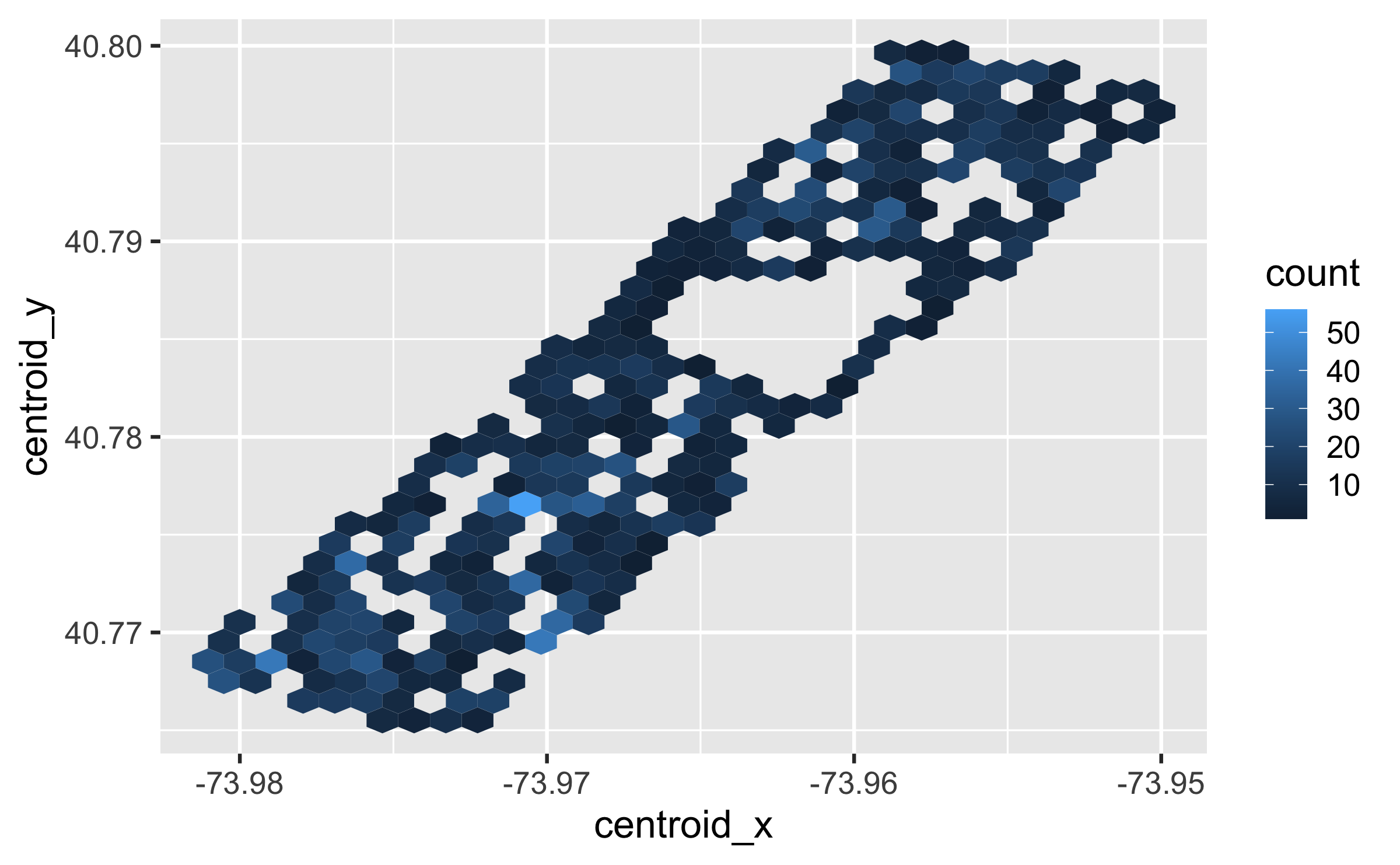
hectare_counts <- squirrels %>% group_by(hectare) %>% summarise(n = n()) hectare_centroids <- squirrels %>% group_by(hectare) %>% summarise( centroid_x = mean(long), centroid_y = mean(lat) )squirrels %>% left_join(hectare_counts, by = "hectare") %>% left_join(hectare_centroids, by = "hectare") %>% ggplot(aes(x = centroid_x, y = centroid_y, color = n)) + geom_hex()The squirrel is staring at me!
squirrels %>% filter(str_detect(other_interactions, "star")) %>% select(shift, age, other_interactions)## # A tibble: 11 × 3## shift age other_interactions ## <chr> <chr> <chr> ## 1 AM Adult staring at us ## 2 PM Adult he took 2 steps then turned and stared at me ## 3 PM Adult stared ## 4 PM Adult stared ## 5 PM Adult stared ## 6 PM Adult stared & then went back up tree—then ran to differ…## # … with 5 more rowsCommunicating for your audience
- Avoid: Jargon, uninterpreted results, lengthy output
- Pay attention to: Organization, presentation, flow
- Don't forget about: Code style, coding best practices, meaningful commits
- Be open to: Suggestions, feedback, taking (calculated) risks